Programming Structural Analysis and Finite Elements in JavaScript

Javascript is an object-based and prototype-based language, and as such the application code is split into various objects containing their properties and methods. This is different to many higher level languages such as Java or C which are class-based.

beam Object (properties)

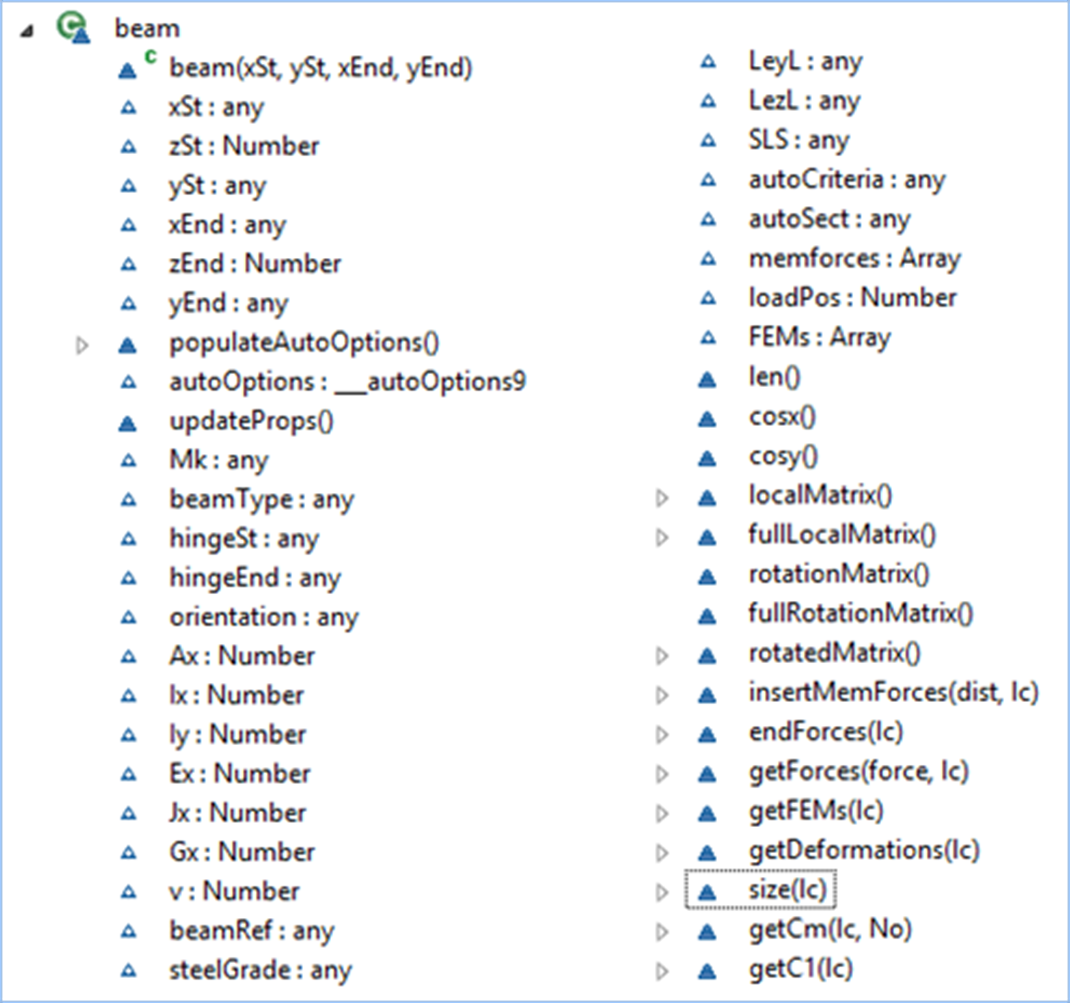
Figure 3‑1 Beam Object UML Diagram Showing Available Properties and Methods

All instances of beam objects are contained within the beams() array.

Beam object has the following properties:

- xSt, ySt, zSt, xEnd, yEnd, zEnd – start and end coordinates, where zSt and zEnd are fixed at 0 for 2D problems.

- Mk – Beam Mark (reference)

- beamType – Type of beam – e.g. "generic", "Steel Section" or "Auto Steel" corresponding to different types of beams that can be inputted. Obviously this can be expanded in the future to include standard materials (steel/concrete/timber) and some standard sections where section properties can be easily calculated (e.g. rectangular, circular, hollow box or circular sections, etc).

- hingeSt and hingeEnd – have a value of 1 or 0 depending on whether a hinge at the end of the beam is present or not.

- orientation -  Orientation of the beam – has a value of 0 if the major axis of the beam lies in-plane (plane frames) or a value of 1 if it is perpendicular to the plane (grillages)

There are further specific properties for different section types. For generic sections, values of A, Ix, Iy, E, J, G and v are inputted manually.

beam Object procedures and functions

Beam is the most complicated object and contains nearly 1/3 of the code of the entire application (1500+ lines of code). It contains a large number of methods that are generally represented by functions and return an appropriate result. All beam methods are listed below. Some are very simple, and their names are generally self-explanatory, whereas the more complex methods will be described in more detail.

this.updateProps - updates member properties from defaults values - normally used whenever a beam object is created.

this.memforces - contains free bending moment diagram and other member forces for a simply-supported member and calculated by the loadVector() function for all member loads during analysis. These are normally modified by the this.getForces function to produce member forces adjusted for fixed-end forces taken from the analysis

this.len - returns the length of the member

this.cosx, this.cosy - returns direction cosines about the x and y axes (direction cosine about the y axis = direction sine about the x axis)

this.fullLocalMatrix - returns a member matrix for a 3D element. Calculates all stiffness coefficients and returns a matrix object. The matrix is adjusted for hinges and also Ix and Iy are inverted for members that are treated as grillage elements (i.e. major axis of a member perpendicular to the x-y plane). A typical matrix for a bar element with no hinges is as follows:

E*A/L						-1*E*A/L
	12*E*Ix /L/L/L				6*E*Ix /L/L		-12*E*Ix /L/L/L				6*E*Ix /L/L
		12*E*Iy /L/L/L		-6*E*Iy /L/L				-12*E*Iy /L/L/L		-6*E*Iy /L/L
			G*J/L						-1*G*J/L
		-6*E*Iy /L/L		4*E*Iy/L				6*E*Iy /L/L		2*E*Iy/L
	6*E*Ix /L/L				4*E*Ix/L		-6*E*Ix /L/L				2*E*Ix/L
-1*E*A/L						E*A/L
	-12*E*Ix /L/L/L				-6*E*Ix /L/L		12*E*Ix /L/L/L				-6*E*Ix /L/L
		-12*E*Iy /L/L/L		6*E*Iy /L/L				12*E*Iy /L/L/L		6*E*Iy /L/L
			-1*J*G/L						J*G/L
		-6*E*Iy /L/L		2*E*Iy/L				6*E*Iy /L/L		4*E*Iy/L
	6*E*Ix /L/L				2*E*Ix/L		-6*E*Ix /L/L				4*E*Ix/L

Table 3‑1 - Element Stiffness Matrix

this.fullRotationMatrix - returns a 3D rotation matrix for an element and use for the rotation of the element stiffness matrix and for coordinate transformations.  All member loading needs to be converted from ‘Local’ or ‘Member’ coordinate system into ‘Global’ coordinate system to form a solution. Similarly, to obtain member forces, the global resulting displacement and member forces are transformed and outputted in Local member coordinates. All angle displacements and moments remain unchanged; whereas vertical and horizontal forces and displacements are multiplied by the sine or cosine of the angle of the inclination of the member α (Transformations are achieved through the application of the principle of contragredience ^{(Jenkins, 1969)}).

Table 3‑2 Graphical Presentation of Coordinate Transformation

this.endForces(lc) - returns member end forces for an inputed load case.

this.getForces = function(force,lc) - returns an array containing moments along the length of the beam, where force=0:axial;1:shears x-x;2:shear y-y; 3:torsion; 4:moments y-y; 5:moments x-x 6:lengths along

this.getDeformations(lc) - returns deformations in all three directions in local member axes. For the inputted loadcase, calculate and sum two components of deflections. The first component obtained by interpolating the end displacements and rotations using the appropriate shape function:

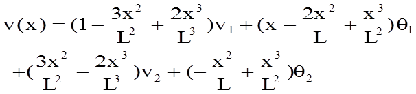
This is based on the information provided within the lecture notes by (Chandra & Namilae, n.d.)

The second component of deflection was originally calculated by integrating the bending moment diagram for an equivalent en-castre member (moment-area theorem) - based on the guidance provided within (Prakash, 1997).

The procedure is carried out twice for both in-plane and out-of-plane deformations and with making allowance for hinged member where appropriate. Because the end-rotation for hinged members cannot be extracted from the displacement matrix directly (as it equals 0 for hinged members), it will need to be calculated when the loadVector is formed. This functionality is yet to be implemented, thus the displacements for hinged members are currently incorrect.

This method has proven difficult to implement for hinged members. Thus a simpler approach of directly calculating member deflections using formulae by the loadvector() function available at http://www.tquigley.com/T312.htm was adopted for the final version.

support Object

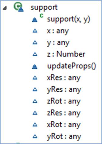
Figure 3‑8 Support Object UML Diagram Showing the Available Properties and Methods

The support object is far less complex than the beam object, and it only contains support coordinates and values of 0 or 1 for each of the restraint conditions.

updateProps() method is invoked when a support object is created to fill in default restraint values.

pLoad Object

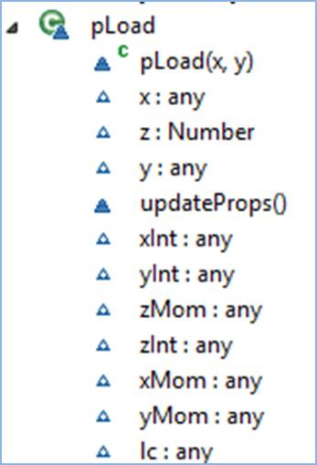
Figure 3‑9 pLoad object - Showing the Available Properties and Methods

pLoad object is not dissimilar to the support object, and only contain properties of inputted point loads. These include load coordinates and intensity as well as the assigned load case (lc).

lLoad Object

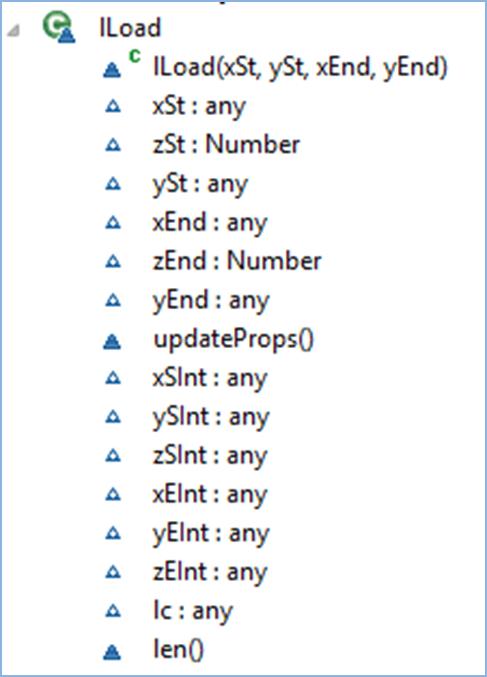
Figure 3‑10 lLoad Object UML Diagram Showing the Available Properties and Methods

lLoad object contains line load start and end coordinates, start and end intensities and the load case.

updateProps() method updates object properties and len() returns the length of the line load.

Structural Analysis

Structural analysis is performed by a series of functions. The code was subdivided into individual functions to simplify debugging and to be able to call up parts of the procedure as required. The analysis utilises the standard stiffness method, and the implementation is loosely based on the Matrix Structural Analysis of Plane Frames using Scilab (Annigeri S, 2009). The publication, which forms a part of Prof Annigeri‘s lecture notes provides extensive guidance on forming the relevant matrices and extracting member forces, and also provides examples which allow for quick verification of the code. The algorithm was adopted for the use in JavaScript with Sylveter Matrix library, and to allow for additional learn7-programming-finite-elements-in-javascript.htms of freedom, hinges, member loads etc. All matrix manipulations were handled by the JavaScript Matrix library Sylvester developed by JC Coglan. The library and API documentation is available at (Coglan, 2007-2012) and handles matrix manipulations such as multiplication, inversion etc.

getNodes function loops all beams and assigns nodes then stores node coordinates and stores them within the nodes() array. In order to establish connectivity between members, each potential new node is checked against the existing array to avoid creating duplicates.

Function locationMatrix() forms the location matrix and calculates the number of learn7-programming-finite-elements-in-javascript.htms of freedom (ndof). It loops all nodes and for each learn7-programming-finite-elements-in-javascript.htm of freedom that is not restrained assigns a consecutive integer within the location matrix. All restrained nodes are assigned a zero within the location matrix. Rows within the matrix correspond to nodes, and columns to learn7-programming-finite-elements-in-javascript.htms of freedom. Thus a typical location matrix for a simply supported beam would be:

[0, 0, 0, 0, 1, 2]
[0, 3, 0, 0, 4, 5]

Note that the structural analysis algorithm allows for potentially 6 learn7-programming-finite-elements-in-javascript.htms of freedom at each node: x-axis translation, y-axis translation, z-axis translation (out of plane), torsional rotation, out of plane rotation and in-plane rotation. This allows for analysis of both plane frames and grillages.

structureSMatrix() function calls up the beam.rotatedMatrix() function for each of the beams (please see previous section) which returns the rotated stiffness matrix and then sums up the appropriate stiffness coefficients to form the structure stiffness matrix. The references to rows and columns within the matrix correspond to integers within the locationMatrix(), and all restrained DOFs are eliminated from the structure stiffness matrix to allow for supports and also to reduce computational workload associated with manipulating the structure stiffness matrix. The function returns a Sylvester matrix object to allow for further manipulation.

loadVector(lc) function is complex as it forms the load vector for any given loadcase, but also stores the relevant free member force diagrams (e.g. free BM diagram), end displacements that are used for displaying member force results. The function loops through all joint loads and then also discretises all line loads into a series of individual point loads (between 41 and 99 depending on the relative length of the line load and the minimum beam length). This forms an allLoads() array. loadVector() function then loops through all loads to find loads applied at nodes. These are immediately inserted into the loadVector array. All loads applied directly on a supported node corresponding directly to the supported DOF are directly saved within the reactions() array and are disregarded from further analysis

Member loads require significantly more attention. Firstly, all loads are rotated into member coordinate system and split into a component perpendicular to the beam and a component along the beam. Out-of-plane loads do not require rotating as these are always perpendicular to the x-y plane (for grillages). The algorithm then calculates the end forces and inserts them into the loadVector. It also calculates free member forces and stores them in beam.memforces for each beam and for each loadcase. The effects of all point loads (or discretised line loads) are summed. Allowance for hinges is also made as required. The algorithm also stores whether all loads are applied within the central ¼ of the beam length so as to be able to select the appropriate Lateral Torsional Buckling coefficients in the sizing algorithm. The function returns a Sylvester matrix object to allow for further manipulation. Because Sylvester library does not work with 0 and 1 element matrices (corresponding to 0 or 1 DOFs), these are treated differently.

Graphical Display and Interaction – Canvas

There are two main ways of displaying and interaction with graphical information on the web currently – Scalable Vector Graphics (SVG) and the Canvas element. Whilst both have their advantages and disadvantages, canvas is a more recent development and has significant performance advantages when dealing with a large number of graphical elements. Generally, SVG keeps graphics in vector format and assigns a DOM reference to each of the new elements, which consumes a lot of RAM and processor resources, but makes it much easier to interact with.

The Canvas HTML element, as its name states, acts as a simple drawing canvas where the graphical information is to be displayed. Once an object is drawn onto the canvas it cannot be addressed any more. This reduces the memory footprint for difficult scenes, but it makes it somewhat more difficult to interact with.

The canvas features its own coordinate system which can be translated, rotated and scaled to suit.

As it is difficult to alter the contents of the canvas, the normal approach is to redraw the canvas whenever the contents changes. This is handled by the redraw() function and normally takes a small fraction of a second. In games, the canvas is usually redrawn 30 or 60 times per second to maintain fluid animation, but this approach is not necessary with this interactive application.

When displaying the main structural elements, the canvas coordinate system is normally scaled and panned so that it matches the global structure coordinate system. The draw coordinates are thus inputted in the global coordinates. On the other hand, when displaying member forces and deformations, the Canvas coordinate system is rotated, translated and scaled to match the local coordinate system of each beam and the forces are plotted directly. Thus, all complex coordinate transformations are handled by the JavaScript engine which runs on native code and is highly optimised and far quicker to execute. It also avoids the need to manually transform coordinates.

At the moment, for input, all clicks are snapped to a major or a minor grid (if either is toggled on), or can be freely clicked. For future development, the UI should be expanded to allow numerical input of coordinates (relative and absolute) and snapping to intersection, end and mid points similar to CAD applications. It is also possible to import member geometry from a DXF file (which can be exported from CAD applications). Imported geometry is snapped to the 0.1m grid by default.

Because the elements are not identified directly, an elaborate technique of using a shadow canvas (a second canvas that is not displayed and only exists in memory) is created to match the main canvas in size. Each of the elements is then plotted onto the shadow canvas and the colour of the clicked pixel is queried until a match is found. This is one of the many techniques used for detecting selections on a canvas and is very versatile as it does not require the clicks to be identified from element geometry and enables the detection of complex objects. The technique is described in detail in the Gentle Introduction to Making HTML5 Canvas Interactive (Sarris, 2011). Detecting double-clicks uses the same technique and facilitates the deletion of elements.