Konstrct.com is a fully web-based structural
analysis tool built using web-technologies incuding JavaScript
and html5. It can be used to perform structural analysis of plane frames
and grillages, and automated steel sizing and optimisation
to Eurocode 3
(EC3).
The application runs within a web browser and are thus fully
portable and compatible with a large variety of devices such a smartphones,
tablets and PCs. This is in contrast to most structural analysis tools in use
today which are often very feature rich and efficient, but remain mostly PC
based.
The application was developed over a period of some three
years and build upon an MSc project in Structural Engineering at the University of Surrey.
The structural analysis utilises the stiffness
method and the application contains an optimisation
tool is based on an iterative technique to select the optimal steel sections
based on the prescribed criteria (minimum weight or section height).
The graphical user interface is
fully html5 and
standards based and the graphical display and interaction was built using the
recently introduced canvas element.
Because it is standards based, the
application was successfully tested on many different platforms including
different PC browsers (Mozilla, Chrome, IE), tablets (iOS and Android) and also
smart phones (iPhone and Android).
Current Limitations and Future Work
The application remains in beta, and more
testing is required to validate many different scenarios that can be analysed.
The application is currently limited to
beam elements only and only allows for linear analysis. The addition of
non-linear analysis and other types of elements which would enable the analysis
of slabs and shells is expected to be introduced in the future.
Whilst functional, the optimisation
algorithm remains somewhat basic, and will not produce a true optimal
solution for problems with a high learn7-programming-finite-elements-in-javascript.htm of static indeterminacy. In such cases
it is likely that the algorithm will lead towards a local minima rather than a
true global optimum as discussed in the Optimisation
section.
By using this software you agree to the terms and conditions
below
THE SOFTWARE IS PROVIDED 'AS IS', WITHOUT WARRANTY OF ANY KIND, EXPRESS
OR IMPLIED, INCLUDING BUT NOT LIMITED TO THE WARRANTIES OF MERCHANTABILITY, FITNESS
FOR A PARTICULAR PURPOSE AND NONINFRINGEMENT. IN NO EVENT SHALL THE AUTHORS OR
COPYRIGHT HOLDERS BE LIABLE FOR ANY CLAIM, DAMAGES OR OTHER LIABILITY, WHETHER
IN AN ACTION OF CONTRACT, TORT OR OTHERWISE, ARISING FROM, OUT OF OR IN
CONNECTION WITH THE SOFTWARE OR THE USE OR OTHER DEALINGS IN THE SOFTWARE.
User Interface – Manual
This application is still in development - use with caution!
Structural software is not a replacement for the knowledge of structural
design.
The application should only be used by a trained, qualified and experienced
engineer or for learning and training. All results must be checked by hand
calculations!
Structural Analysis EC3 Sizing+Optimisation Application for html5 and
JavaScript
Copyright (c) 2011-2014 Marko Nesovic, all rights reserved
Brief Instructions:
-You need at least some beams, some supports and some loads to run analysis
-To delete elements, double-click on them
-To improve performance use few auto-size members and fix the size of as many
beams
as possible by changing their type from auto to steel section
If you have any comments, please contact me on konstrct (at) outlook . com
By using this software you agree to the terms and conditions below
THE SOFTWARE IS PROVIDED 'AS IS', WITHOUT WARRANTY OF ANY KIND, EXPRESS
OR IMPLIED, INCLUDING BUT NOT LIMITED TO THE WARRANTIES OF MERCHANTABILITY,
FITNESS FOR A PARTICULAR PURPOSE AND NONINFRINGEMENT. IN NO EVENT SHALL THE
AUTHORS OR COPYRIGHT HOLDERS BE LIABLE FOR ANY CLAIM, DAMAGES OR OTHER
LIABILITY, WHETHER IN AN ACTION OF CONTRACT, TORT OR OTHERWISE, ARISING FROM,
OUT OF OR IN CONNECTION WITH THE SOFTWARE OR THE USE OR OTHER DEALINGS IN THE
SOFTWARE.
The user interface enables
rapid development, testing and validation of the application. The UI enables
graphical input of data (beams, supports and loading) as well as the graphical
output of results.
The user interface is fully HTML5 based and include standard
HTML elements, whereas a canvas graphical element (new to HTML5) is used for
the display of graphical information and for graphic input. Interactivity is
provided through JavaScript, which provides both interaction with forms and
buttons as well as drawing within the canvas element and interactivity within
the canvas. Konstrct.com utilises twitter bootstrap to improve the visual
quality of the application and provide the necessary scalability for various
screen sizes.
Visually, the aim was to keep the layout as simple as
possible whilst providing all the required functionality. This was done so that
the application does not appear cluttered and daunting to potential novice
users but still enabling access to finer levels of input and accurate
structural modelling and sensible sizing of structural elements.
The UI was structured to enable the application to be used
both on a PC with keyboard and a mouse and on touchscreen phones and tables
(iOS or Android based). It was tested in Mozilla Firefox, Chrome and Internet
Explorer (later versions enabling HMTL5 support). No major incompatibilities
between different systems were encountered.
As with most structural analysis applications, the UI is
split into two main elements – input of data and output of results. The main
input screen enables the user to select elements (in order to edit their
properties) or delete them by double-clicking or double-tapping. It also
enables the user to input the general information about the project such as
name, ref number etc.
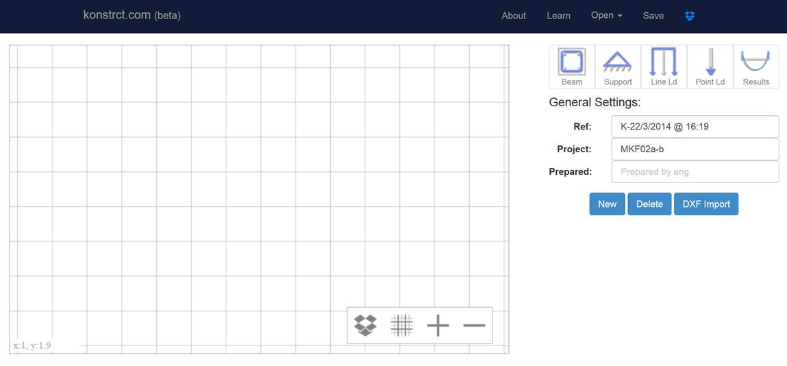
Figure 3‑11 - Main input screen
The structural elements available for input include beams,
supports, line and point loads. All are inputted graphically by clicking on the
main drawing canvas. By default a 1m major grid is enabled and all clicks are
snapped to it. It is possible to turn it off and a 0.1m minor grid is also
available for higher precision. The canvas can be zoomed in and panned. Using
the minor and major grid as well as zooming and panning, it is possible to
easily input and model various structural problems with 0.1m accuracy either on
a PC or on touch-screen devices.
Numerical data/properties are inputted through a table/form
displayed on the right hand side of the screen. The contents of the form
changes to suit the currently selected element. Also, for beams, the form
changes to accommodate different types of input required for defining different
types of beams. Please see the forms reproduced below.
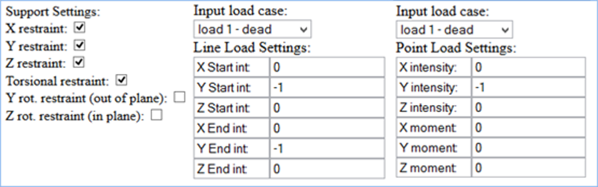
Figure 3‑12 Supports and Loading Input Forms
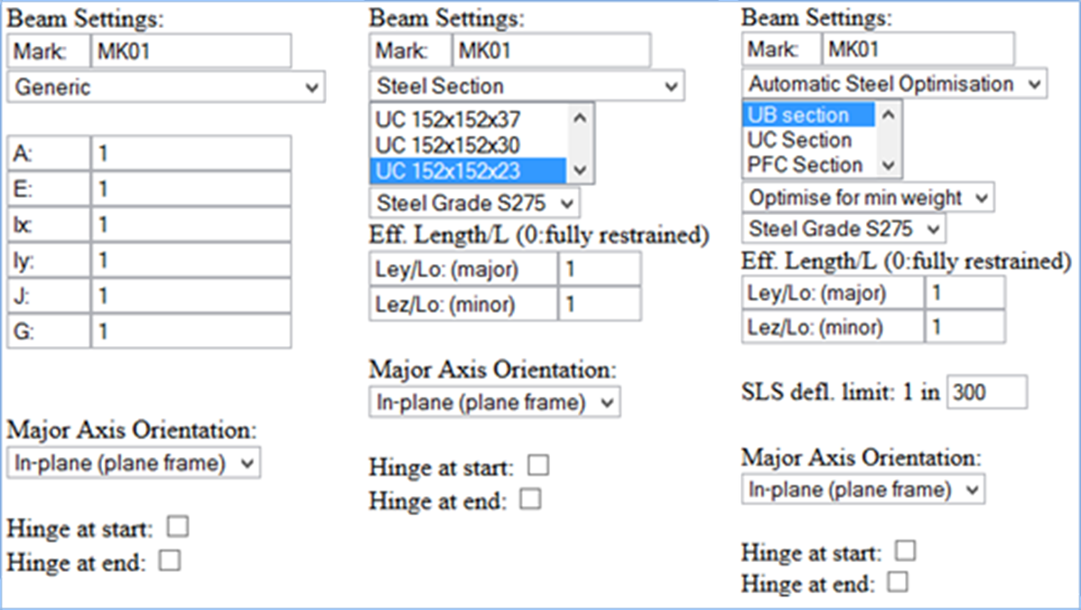
Figure 3‑13 Beam Data Input Forms
The application provides the following output:
- a. AxialForces
- b. Shear
Forces (in-plane)
- c. Shear
Forces (out-of-plane)
- d. Bending
Moments (in-plane)
- e. Bending
Moments (out-of-plane)
- f. Torsion
- g. Deformations
(in-plane)
- h. Deformations
(out-of-plane)
- i. Reactions
- j. Matrices:
- i. Structure Stiffness Matrix
- ii. Location Matrix
- iii. Load Vector
- iv. Member Matrices
- v.Global Displacement Matrix
- vi. Member End Forces
(n.b. matrices are
outputted with the selected input load case to enable output of lower level
data such as member matrices, etc)
- k. Member Sizing
A single screenshot is presented below showing a typical
bending moment diagram for a portal frame subject to a point load at mid-span.
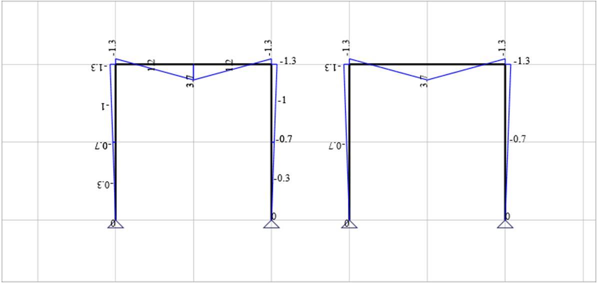
Figure 3‑14 Typical Output Diagram (BM diagram)
Treatment of frames and grillages
The main plane of the screen is treated as an x-y plane, and
the z axis is taken to be perpendicular to it. Loading can be inputted in all
three axis and results can be obtained in-plane and out-of plane. This enables
the analysis of both plane frames and grillages depending on how data is
inputted.
If loads are only inputted in the x and y axes, then the
problem is a plane analysis case, and the user should only seek in-plane
results. On the other hand, if loading is inputted in the z-axis, then the user
should look at out-of-plane member forces. Obviously, it is possible to combine
both and get results in both directions to analyse, for example, a frame
subject to both vertical (gravity) and out-of-plane lateral loading (e.g.
wind).
A switch within the beams input form allows the user to set
the orientation of the beam, or more precisely, select whether the major axis
of a beam sits in-plane or out-of-plane.
Structural Analysis Software and Methods
Structural analysis tools have been created ever since the
development of early computers because these allow for rapid solution of
complicated structural problems in the fraction of the time required to do hand
calculations. The initial tools were very basic in both functionality and
performance offered by the computers in the past. However, over time,
comprehensive software was developed, and modern structural applications now offer
full analysis, design and optimisation solutions helping engineers rapidly
prepare designs of very complex structures. The advances in structural analysis
now enable engineers to analyse structures that even 15 years ago would not
have been possible to model and design accurately. Most of the existing tools
were developed in low-level languages such as Java or
C++ and remain PC based.
When looking at the literature on computer based structural
analysis and the stiffness method a lot of guidance and code is available in
Fortran, Basic, C and Java.
Software developed using these programming languages is tied to the hardware
and the operating system that it has been compiled and developed for and
porting such applications to different platforms is often very difficult.
A good number of Java based structural analysis tools have
also been developed in the past and some books have been published on the
topic. Whilst significantly more portable, Java applications require that a Java
Virtual Machine (JVM) be installed on the computer to be able to run which can
be cumbersome, and many user choose not to (or don’t know how to) have it
installed. There is a wealth of information on programming structural analysis
software in Java, and a book Programming Finite Elements in Java (Nikishkov, 2010) provides extensive guidance. Some of the chapters from this book can be
applied to this project.
There are many structural analysis (and design) packages
available on the market. Unlike many markets where individual players have
managed to achieve very large market share, and set their software as de-facto
industry standards, the market for structural analysis software is still very
much fragmented with many options available. In addition, many larger practices
still maintain and develop their in-house structural software.
Most of the original software developed in the 80s was very
basic, had non-existent or very basic graphical output and often only textual
data input and included a very limited array of elements. The 90s saw the
development of full graphical interfaces that allowed for much easier modelling
of structures. The functionality of software was expanded to include non-linear
analysis, flexible supports, movable loads, load combinations, etc. The
software popular at the time included SAAP, STAD and many others.
In the past 10 years, the development in commercial software
has concentrated mostly on improving the usability and functionality of the
software, with features such as solids and slab analysis (incl. plate and solid
elements) and dynamic analysis of structures becoming standard in many packages
(although rarely at entry-level prices). Furthermore, most packages have been
expanded to include element sizing and design (in steel, timber, RC) and often
allow some form of graphical output into CAD. Building Information Modelling
(BIM) has saw great expansion and adoption in the past 2-3 years, and the
latest tools from Autodesk and Bentley tie into their BIM systems allowing for
improved cooperation between various disciplines involved in the design of a
building. A short table listing some of the currently popular software listing
their functionality is included below:
Software
Licence
Developer /Publisher
Platform
Capabilities
Commercial
Autodesk
PC, Mac
Structural modelling + analysis of structures; Full BIM
support to integrate with other disciplines; Design and drafting tools
Commercial
Autodesk
PC + cloud storage
Revit add-on; Performs analysis off-site in the cloud to
boost performance. Requires PC structure to input data and view results
Commercial
Autodesk
PC
A popular and feature-rich analysis and design package
incl. non-linear analysis, dynamic analysis, many types of elements, etc.
Links with Revit;
Commercial
Bentley
PC
Full-featured structural analysis tool which includes
non-linear analysis, dynamic analysis etc. Links with RAM and ProSteel for
steel sizing and detailing and with Bentley’s BIM tools.
Commercial
CSI
PC
One of the most comprehensive 2D and 3D structural
analysis packages. The interface is difficult to master for new users, but
functionality is comprehensive. Extensive choice of 1D, 2D and 3D elements
and analysis modes.
Commercial
Dassault Systemes
PC / Windows
supports multiple stages of product development (CAx),
including conceptualization, design (CAD), manufacturing (CAM), and
engineering (CAE).
Commercial
Radimpex
PC / Windows
Offers 3D analysis of linear and plate elements;
Non-linear and dynamic analysis. Concrete, steel and timber sizing to many
codes. Links to proprietary steel and RC detailing tools.
The list above is by no means extensive or complete. Another
non-complete list of finite element packages is available on Wikipedia
(Wikipedia, 2013).
A recent trend in software development in general is to
create web-based
applications that utilise JavaScript scripting language combined with html5
markup language. Whilst more resource intensive than natively compiled
applications these allow for great hardware and software portability and are
capable of running in most modern browsers and can easily be compiled into
full-fledged applications for iOS, Android and Windows 8. In particular, the
introduction of the Canvas element and SVG (Scalable Vector Graphics) in the
recent years has enabled the development of graphics-rich web applications
making it possible to create web-based full-featured structural analysis tools
which require graphical input and representation of results.
The author has not been able to find any purely web-based
structural analysis tools, however good examples of fully web-based
productivity tools include Google mail and docs, Microsoft’s Office 365 (Office
web apps), Apple’s iWorks, and AutoCAD WS. Such application run within a
web-browser and store the information in a cloud making it available from a
variety of devices and allow for very easy access.
Structural Analysis Methods
A Wikipedia definition of structural analysis states: “Structural
analysis is the determination of the effects of loads
on physical structures
and their components. “ (Wikipedia, n.d.). It also
provides a very good Timeline
showing the historical development of structural analysis methods.
Whilst simple single beam and small assembly problems can be
solved directly, the analysis of structurally
indeterminate structures is more complex. There are three main approaches
to solving linear, elastic frame analysis problems. These are Flexibility Method, Stiffness Method, and a particular variation of stiffness
method – Moment
Distribution.
Of the three methods, all have their advantages in
particular situations, and for solving particular problems. The Flexibility method
is particularly useful in solving problems that include frames with a low
learn7-programming-finite-elements-in-javascript.htm of static indeterminacy. The Stiffness method
is suitable for hand calculations where structure has a lower learn7-programming-finite-elements-in-javascript.htm of
kinematic than static indeterminacy. Moment distribution is a widely used and
convenient method for solving complicated problems without the need to set up a
large number of simultaneous equations. It is also a convenient method of
checking computer output.
Konstrct.com
utilises the stiffness methods to resolve
deformations and member forces within the analysed structure. Thus, the
documentation available here concentrates on detailing this method.
Stiffness Method and Finite Elements
Due to the ease of implementation, computational efficiency
and the proven track record, the Stiffness Method is
most commonly utilised in computer applications and is the method used
implemented in the developed application. Over the years Matrix Structural Analysis
has morphed with the Finite Element Method to become the de-facto standard for
computer Structural Analysis tools (Felippa, 2000), with very few tools developed
utilising different methods.
The general procedure for solving structural problems using the
Direct Stiffness Method
is as follows:
1) Establish the number of unknown joint displacements to define the scale of the problem.
2)A number of restraints are introduced to create a kinematically determinate structure
(primary structure), and Member forces for this structure are then found
forming a particular solution for each of the elements.
3) The
structure stiffness matrix K is formed by assembling the element stiffness
matrices/coefficients and the load vector P is formed by finding the equivalent
joint forces.
4)The
complimentary solution is a set of forces required to remove the restraints and
re-establish equilibrium. Finding these forces is normally a two-step process. Initially,
joint displacements are found by solving the equation d = K-1P,
where P is a load vector, K is a structure stiffness matrix, and d is a
displacement vector. Joint displacements are considered the primary solution to
the stiffness method problem. Based on the joint displacements, it is possible
to calculate the member forces due to those displacements using the equation P
= Kd.
5) Finally a
total solution is found: Total Solution = Particular Solution + Complementary
Solution.
Structural analysis and the stiffness method is a
well-established subject with numerous textbooks published on the topic. It is
studied as a part of all undergraduate and post-graduate civil and structural
engineer courses. The recent research on the topic is mostly concerned on
introducing new types of elements, non-linear analysis, dynamic analysis and
optimisation of the calculation method, but these are mostly beyond the scope
of this project.
The
Finite Element Method (Zienkiewicz & Taylor, 2004) is possibly the most
comprehensive textbook on the subject and contains a wealth of information not
available in other publications, however it is very broad. Although an older
book, and not republished recently, (Coates, et al., 1987) provides an
excellent introduction to structural analysis and also gives guidance on
computer applications in structural analysis and was used in developing this
application extensively. This is omitted from many modern textbooks, as most
new engineers elect to use off-the shelf analysis packages. The book still
remains a recommended textbook by many lecturers of structural design.
The essential sources of information are the Lecture Notes
for the Structural Mechanics and Finite Elements module (Sagaseta, 2012). For
this particular project it provides a useful introduction to the stiffness
method as well as detailing many mathematical concepts (coordinate
transformations, shape functions, etc) required to successfully tackle a
project of this type. Furthermore, many lecturers have published their lecture notes on
the internet (Gavin, 2009), (Chandra & Namilae, n.d.), (Felippa, 2004) and many others, and these provide different viewpoints on the similar subject
and expand on the basic syllabus in different ways.
Although the core procedure is common for both
hand-calculations and for computer programme, there are a number of differences
along the way. These all reflect the differences in the ability of an engineer
to selectively apply simplifications and of computers to perform a large number
of calculations quickly and accurately.
Firstly, in hand calculations all axial strains in the
members are usually disregarded. This is a valid assumption, as they contribute
very little to the actual displacements. This assumption is used to reduce the
number of displacements to be considered in hand calculations. However, in computer
software, all displacements are taken into account to simplify the calculations
procedure and the extra computational requirements are normally not an issue
with modern computers. These differences are illustrated below.
Only a brief introduction to the stiffness method is
presented here. The details of the programmatic implementation, as well as a
more detailed description of the method and the techniques employed is detailed
in other chapters.
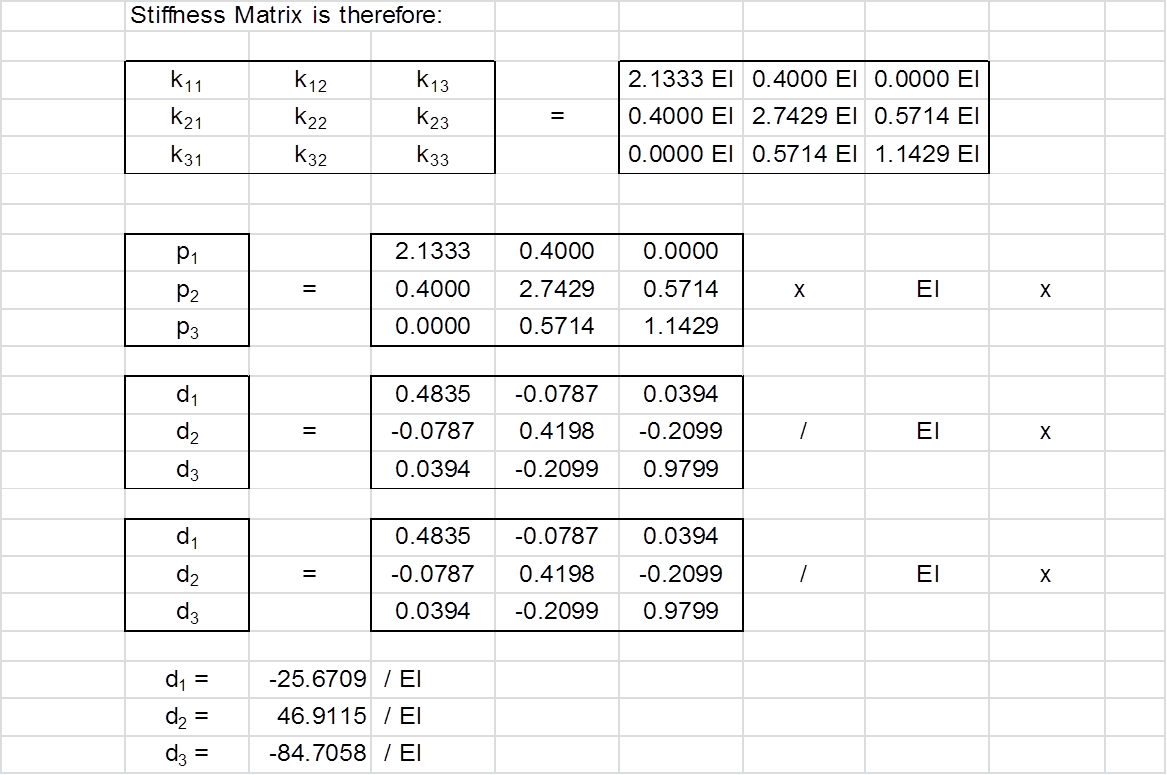
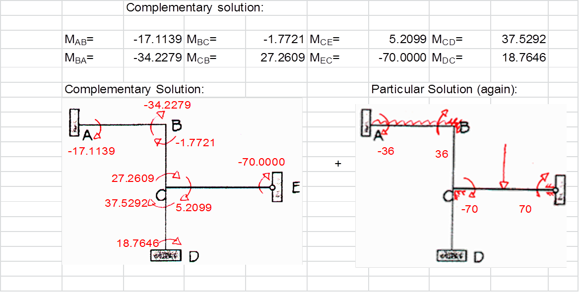
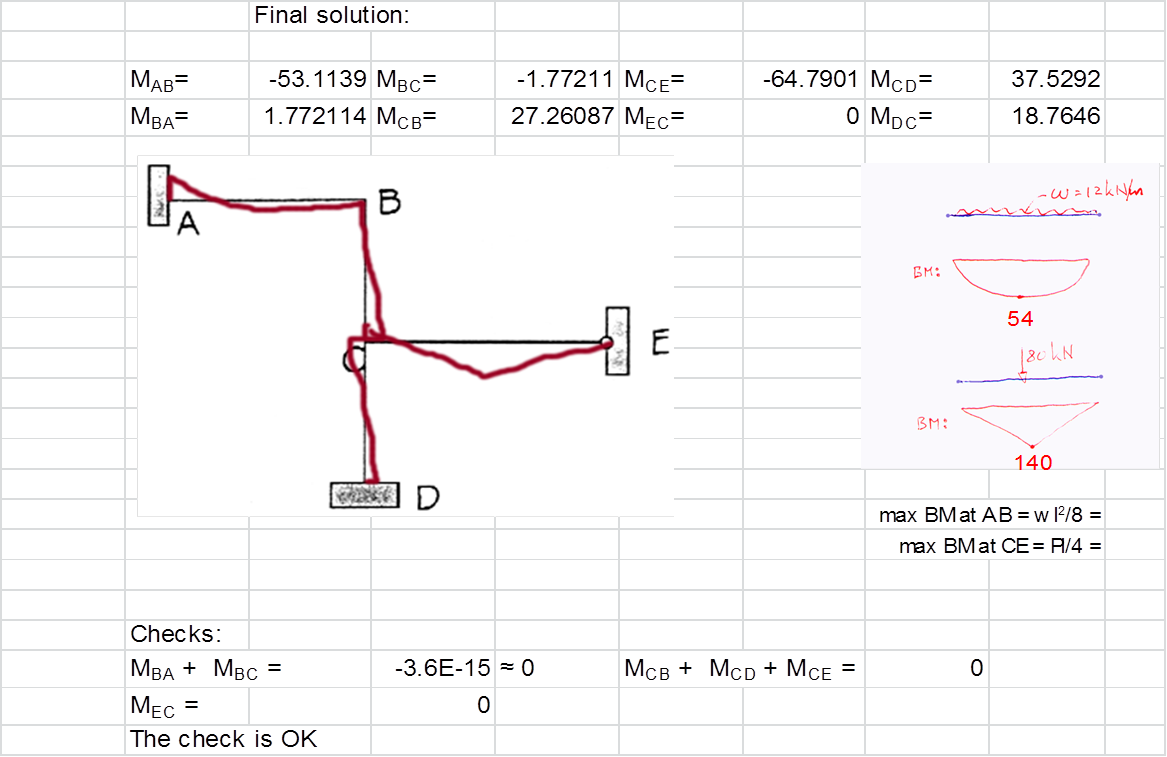
Structural Analysis – Example Hand Calculations
In order to demonstrate the utility and validity of the
application’s structural analysis algorithm a check was carried out against the
simple example hand calculations. The example was part of a 2nd year
structural analysis coursework at Kingston University.
The simplified excel-based calculations is reproduced below.
These are based on the first principles of Structural Analysis and the
Stiffness Method.
Steel Design to Eurocode 3 (EC3)
In terms of structural engineering, Eurocodes are a relatively new
development. These were introduced and first drafts published in the 1990s, and
a full set of codes was finalised and published in 2000s. The structural code
EN 1993-1-1: General rules and rules for buildings for the design of steel
structures (CEN, 2005) was approved by the European Committee for
Standardization (CEN) on 16 April 2004.
The condensed Eurocode 3 (Brettle & Brown, 2009) contains
the very good and extensive design guidance provided in a readable form. The
book is accompanied by two further publications containing worked examples for
open and hollow sections to EC3 which were crucial in validating the code of
the developed application: (Brettle & Brown, 2008) & (E & Brown, 2009).
Appendix A of the Concise EC3 contains design procedures for
various design problems, which provide the basis of the sizing algorithm
implemented within this application. These contain the basic sequence of sizing
checks required to size steel beams in accordance with EC3 and help guide both
engineers and developers of sizing tools. The code within the application which
is detailed further in the following chapters closely follows these diagrams,
and these are thus reproduced below:
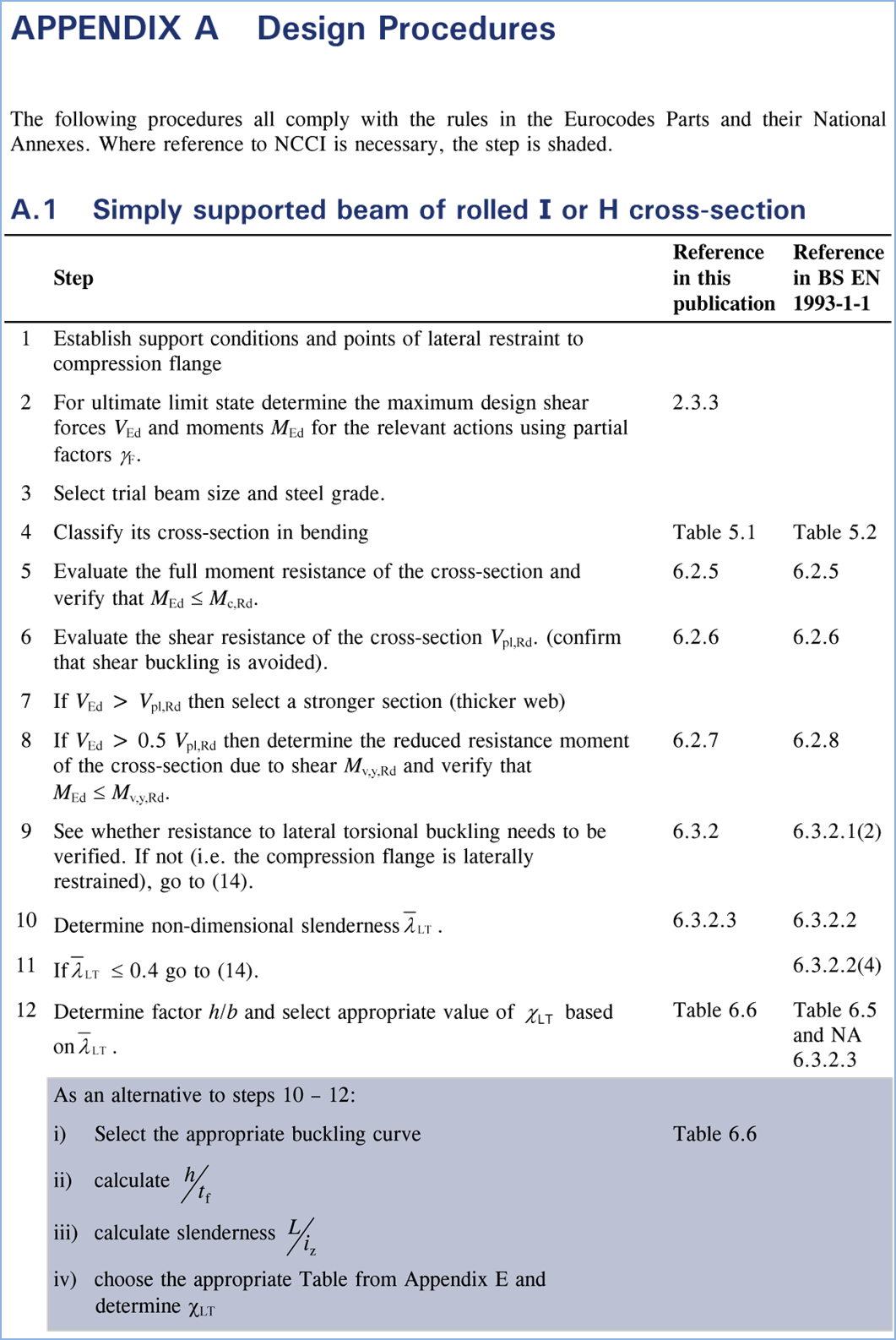
Figure 2‑1 Condensed EC3 Appendix A - Design
Procedures (Brettle & Brown, 2009)
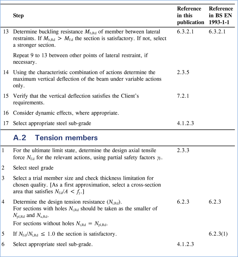
Figure 2‑2 Condensed EC3 Appendix A - Design
Procedures (Brettle & Brown, 2009)
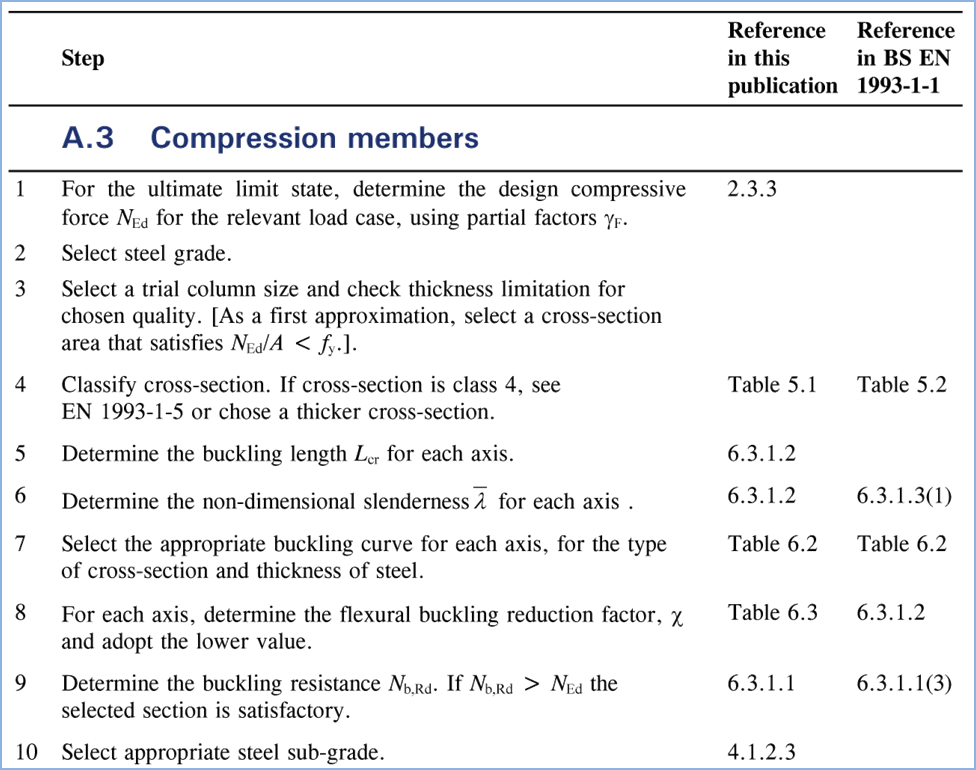
Figure 2‑3 Condensed EC3 Appendix A - Design
Procedures (Brettle & Brown, 2009)
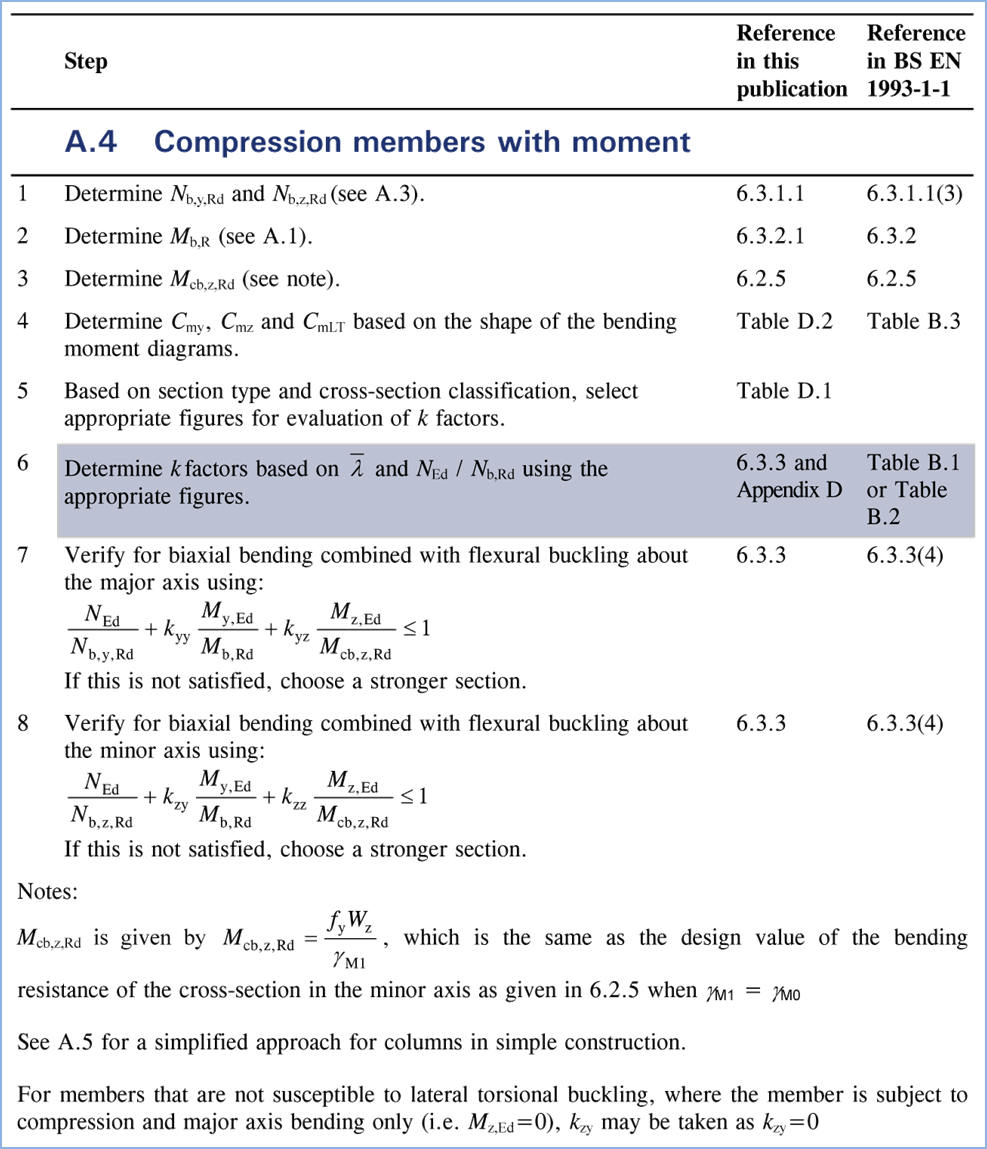
Figure 2‑4 Condensed EC3 Appendix A - Design
Procedures (Brettle & Brown, 2009)
The application utilises these algorithms to perform steel
sizing and also to verify Ultimate Limit State (ULS) capacity of sections as
part of the optimisation procedure.
A publication (jointly published by the The Steel
Construction Institute, Tata Steel & The British Constructional Steelwork
Association Ltd., 2011) contains a wealth of additional information about
various less frequently encountered problems within steel design not contained
within the Concise Euro code or within the actual code. The publication covers
issues such as torsional and torsional-flexural buckling of non
doubly-symmetric sections which are only briefly mentioned within the concise
eurocode and the code itself but were required for the development of the
application which has a broad field of use.
Very little guidance for obtaining the Lateral Torsional
Buckling Factors C1 & C2 is contained within the eurocode. These are very
important in finding the LTB resistance of a member (Mcr). A such, a non-contradictory
complementary information (NCCI) was published (Bureau & Galea, 2010)
providing the additional guidance incl formulae and diagrams.
The application interpolates the values provided within the
diagrams in figures 3.3 and 3.5 from the NCCI to find LTB factor C1. Figure 3.3
is reproduced below, whereas other diagrams can be found within the
publication.
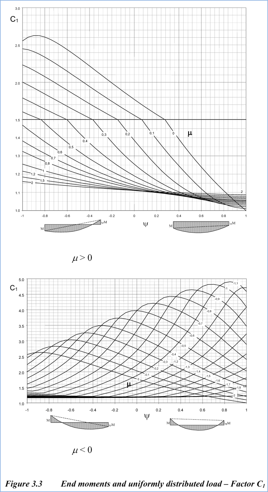
Figure 2‑5 Figure 3.3 showing the values of C1 reproduced
from the NCCI (Bureau & Galea, 2010)
Finally, the blue book has always been the necessary tool
used by steel designers. It contains numerical tabulated geometrical data about
the available steel sections as well as the calculated bending moment capacity
and lateral torsional moment resistance (based on length). The new interactive bluebook
was recently updated in accordance with EC3 and is hosted and published by Tata
Steel and available online (Tata Steel, n.d.). The published section geometry
information was used within the tool.
Beam Sizing to EC3 – Implementation within
konstrct.com
The sizing algorithm is based on the information contained
within EC3 (CEN, 2005),The Concise Eurocode 3 (Brettle & Brown, 2009) and
the associated Examples (Brettle, 2009), (Brettle & Brown, 2008). The
concepts and the contents of these publications is presented above.
The actual implementation of the procedure is presented in a
series of diagrams contained in the following pages. Note that the procedure is
very complex and contains a large amount of checks. For simplicity some of the
less commonly utilised checks have not been presented in the diagram. The
reader is referred to the publications listed above and the actual code of the
application.
As a brief overview, the procedure initially assembles the
relevant factored, ultimate member forces for each element and reads the
element properties. At this stage it also performs the initial capacity checks
(eg P/Afy; M/Wel, etc) to quickly discard substantially undersized sections
and save processing time. Using these checks the algorithm also determines
which detailed checks are required to be carried out. If the applied axial
force and bending moment are within 0.5 or 1% of the capacity, detailed checks
will not be carried out to optimise the output and avoid displaying unnecessary
checks. The procedure then checks shear capacity, axial capacity and bucking,
bending moment and lateral torsional buckling and finally carries out combined
bending moment and axial capacity checks (all if required).
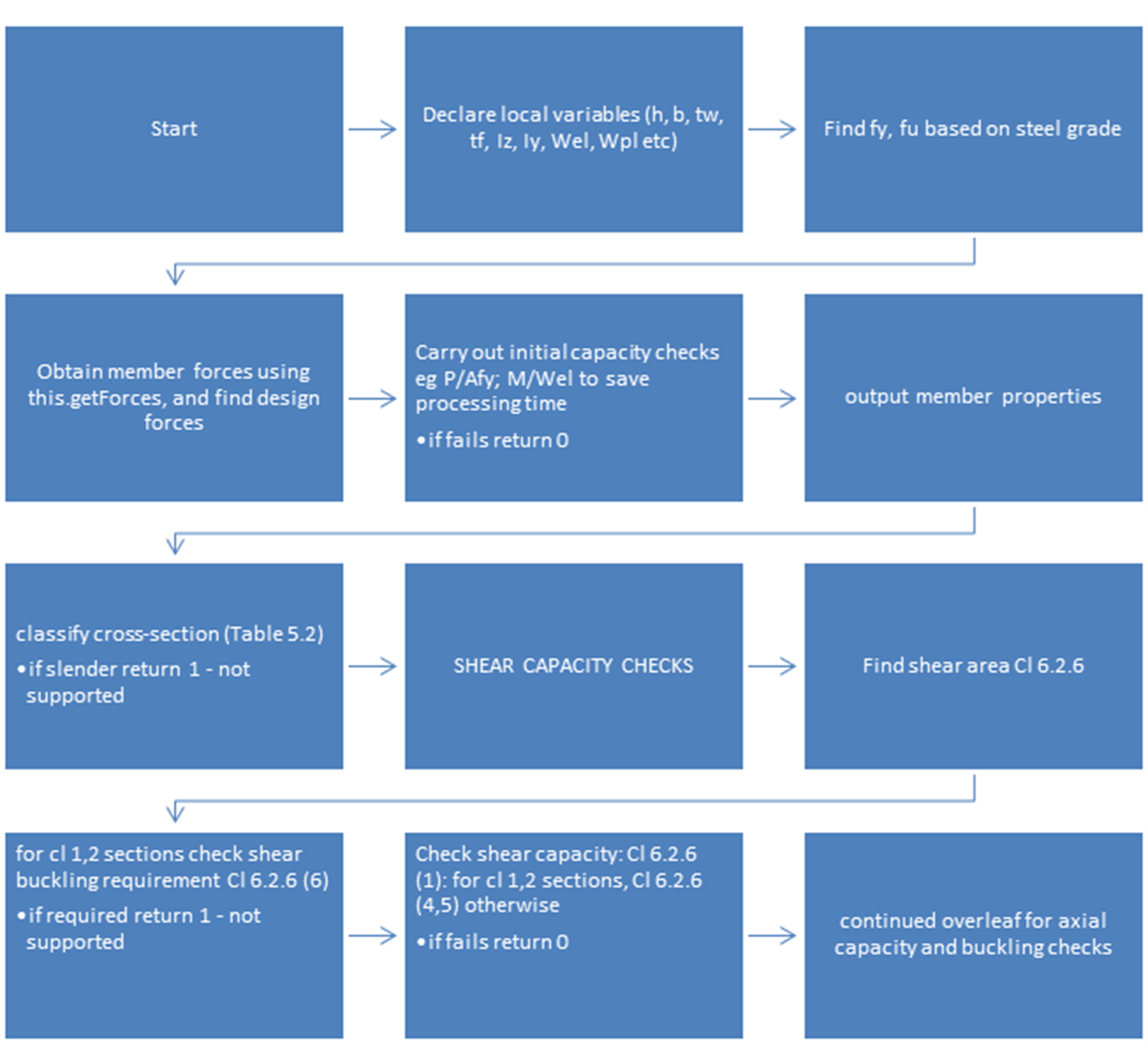
Figure 3‑2 Beam Sizing Algorithm Pt 1/4 – Input data,
Classification, Shear Capacity (CEN, 2005)
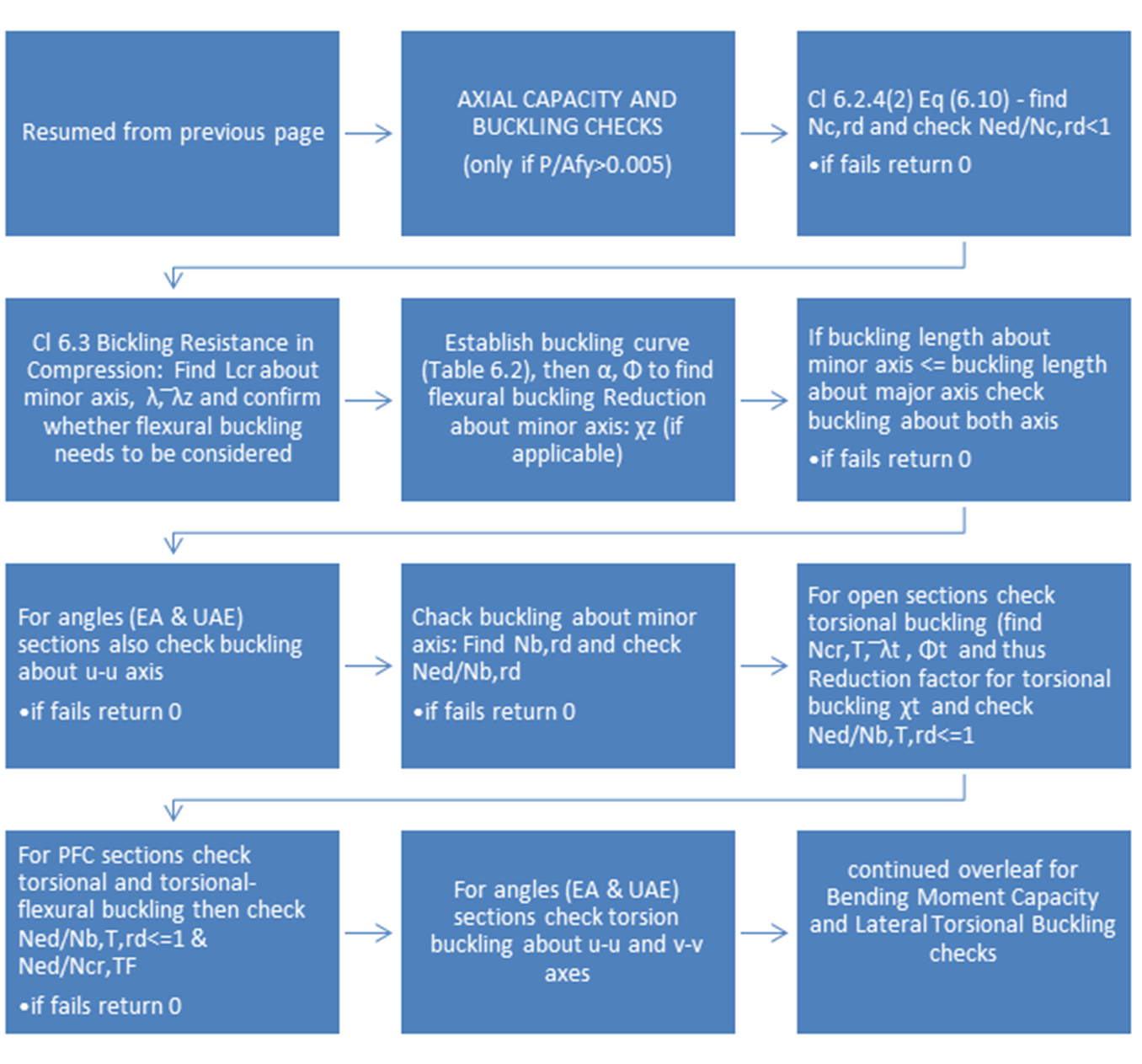
Figure 3‑3 Beam Sizing Algorithm Pt 2/4 – Axial
Capacity and Buckling (CEN, 2005)
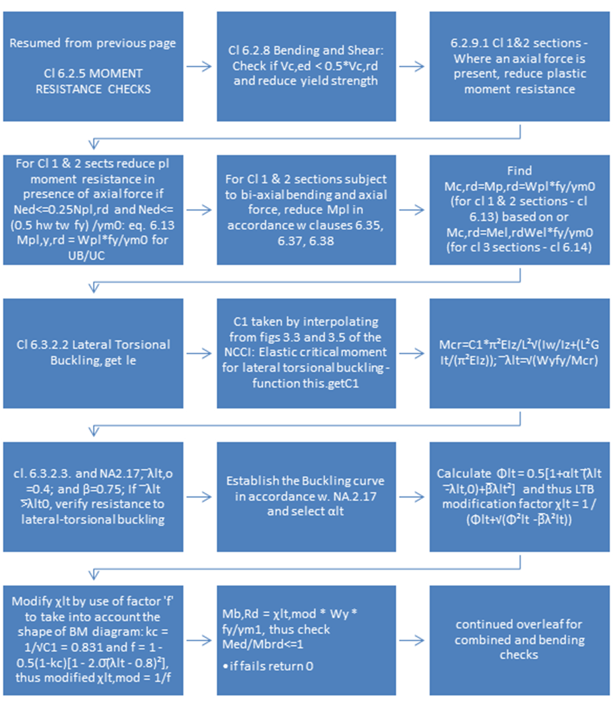
Figure 3‑4 Beam Sizing Algorithm Pt 3/4 – Bending
Moment Capacity and Lateral Torsional (CEN, 2005)
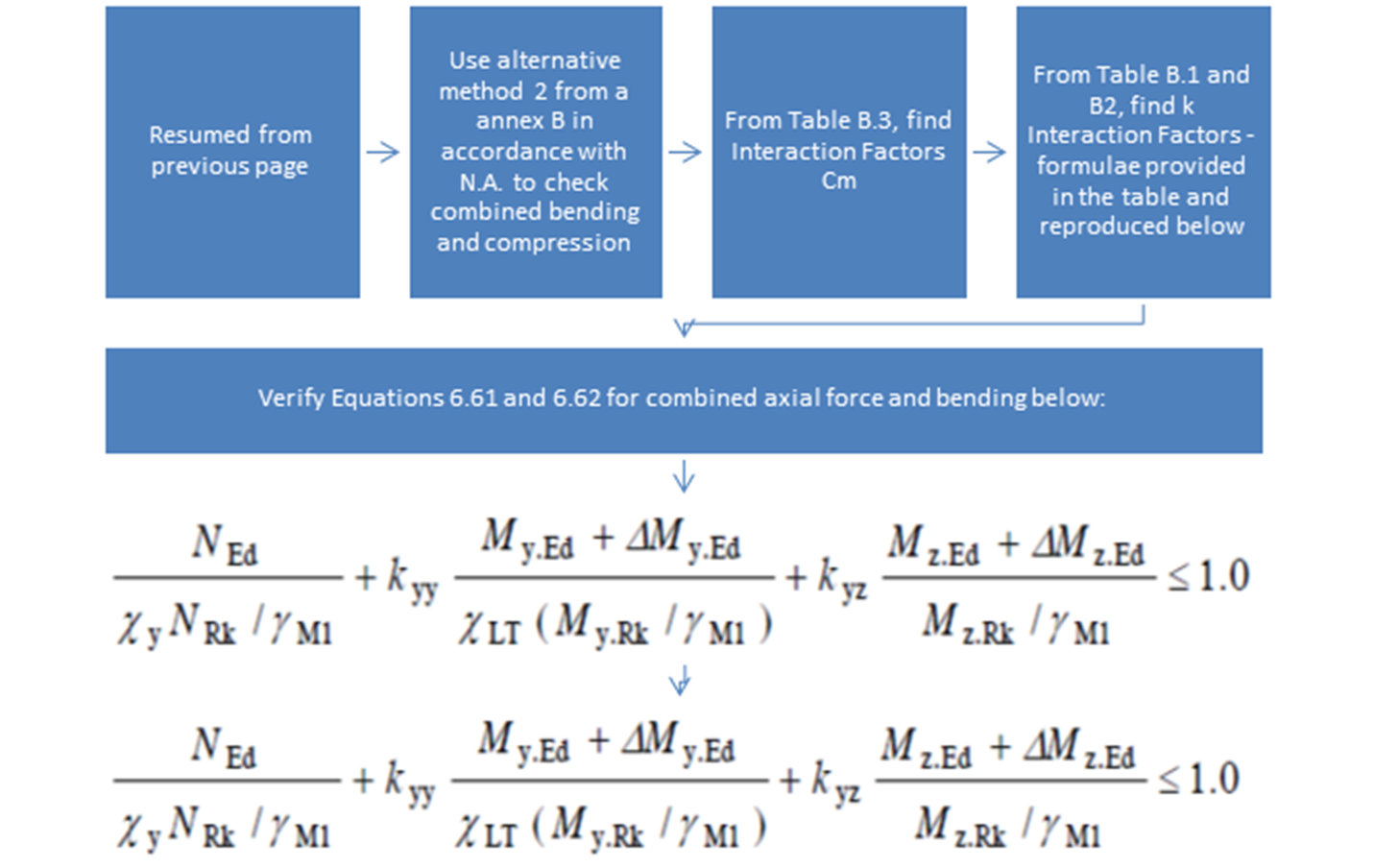
Figure 3‑5 Beam Sizing Algorithm Pt 4/4 – Combined
axial and bending checks (CEN, 2005)
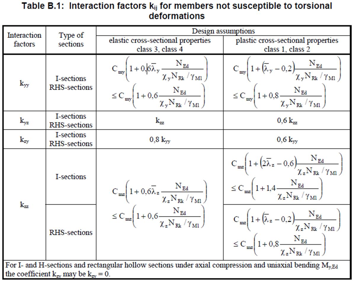
Figure 3‑6 - Interaction Factors kij (CEN, 2005)
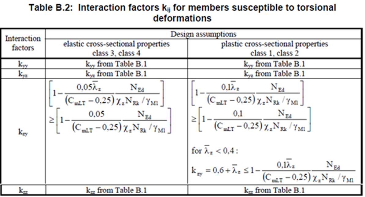
Figure 3‑7 – Interaction Factors kij (CEN, 2005)
Example beam calculations to EC3 reproduced from (Brettle, 2009)
In order to validate the steel sizing
algorithm, a number of checks against the published example 12 within (Brettle, 2009) which provides worked examples for many typical sizing
problems. Example 12 details of sizing for a major axis bending and compression
of Class 3 section which fairly complex including buckling, lateral torsional
buckling and a combined axial force and bending.
Several key sections from the publication
have been reproduced below for comparison and also provides some graphical
data:
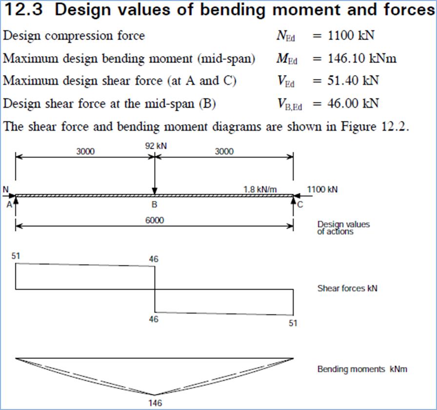
Figure 5‑17 – Steel Building Design, Worked Example
12, Sheet 2/14 - Design Forces (Brettle, 2009)
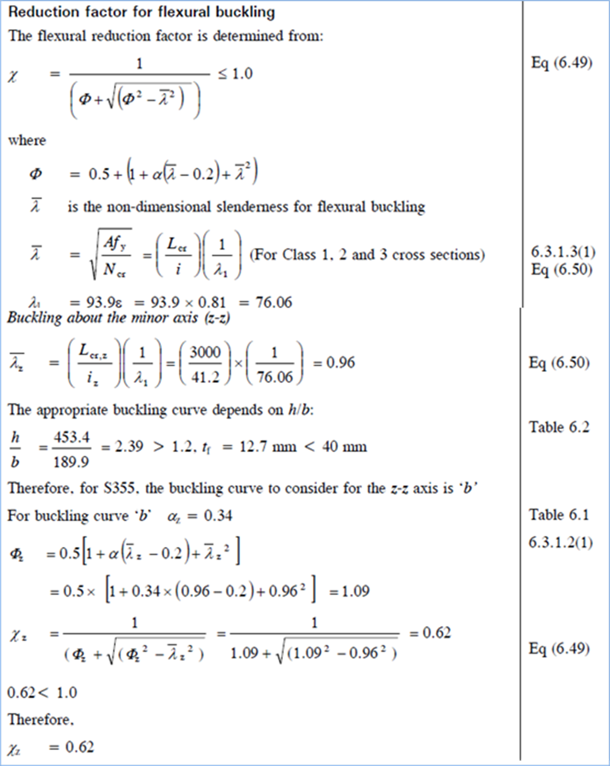
Figure 5‑18 Steel Building Design, Worked Example 12:
Sheets 7&8/14 - Buckling about minor axis (Brettle, 2009)
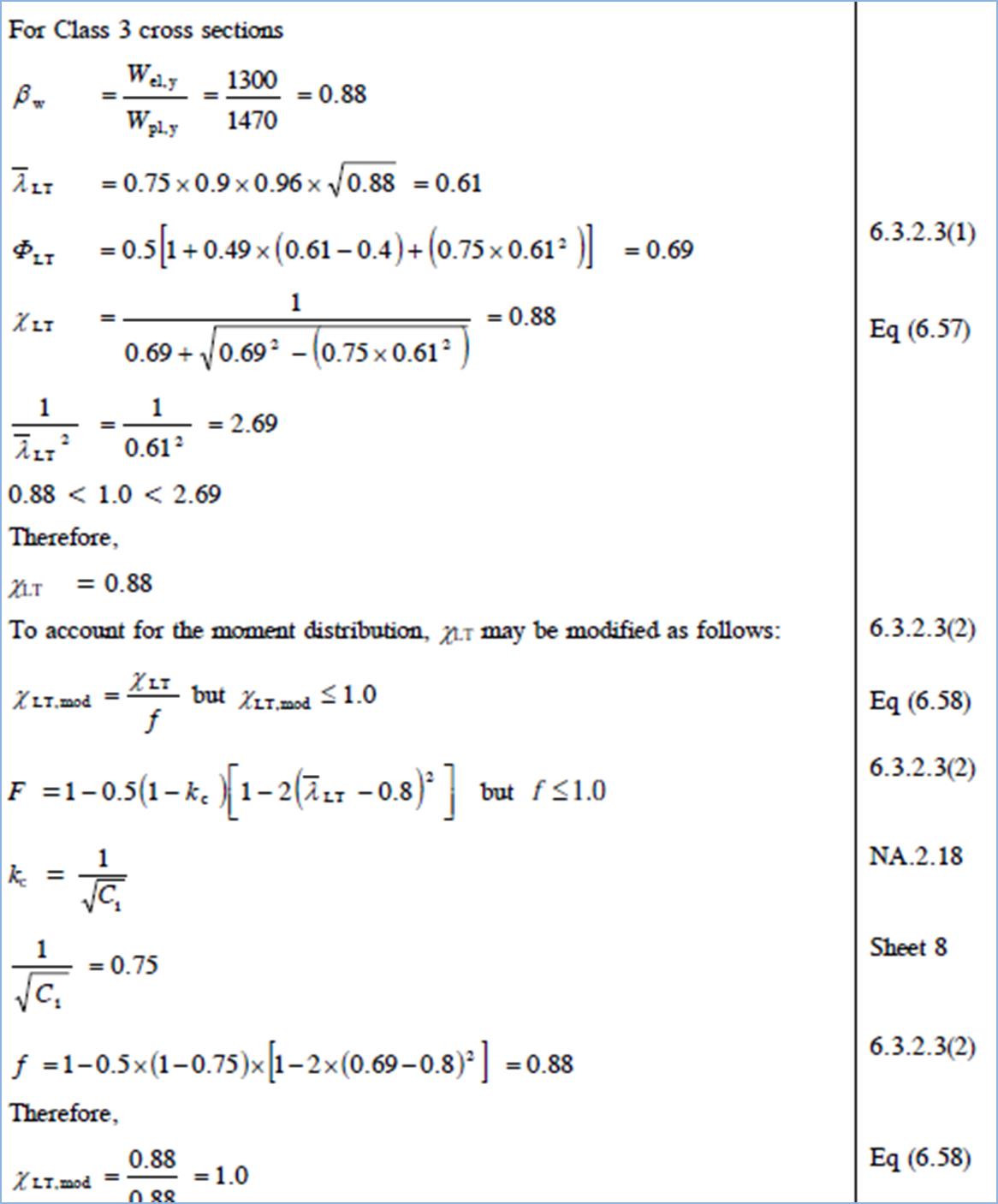
Figure 5‑19 Steel Building Design, Worked Example 12:
Sheet 9/14, Lateral Torsional Buckling Reduction Factor (Brettle, 2009)
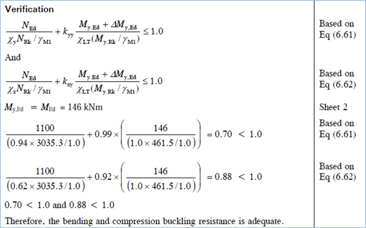
Figure 5‑20 Steel Building Design, Worked Example 12
- Sheet 11/14 - Final Verification (showing k factors) (Brettle, 2009)
Structural Optimisation
Structural
optimisation is an integral part of structural design.
Every engineer should aim to develop the most cost-effective solution to a
given engineering problem. As such computer optimisation techniques have been
developed for a long time in an attempt to automate this process. Some authors
have attempted to utilise standard optimisation techniques taken from
management and industrial optimisation textbooks, whilst others have relied on
iterative techniques more similar to how structural solutions are developed in
a design practice.
(Christensen PW, 2008) provides a good introduction into the
problems of structural optimisations, explaining the main concepts and
providing good guidance on the mathematical methods employed in solving basic
optimisation problems. It discusses the problems of numerical and shape
optimisation, but concentrates mostly on mathematical approaches to numerical
optimisation. Simple Structural Optimisation (SO) problems can be represented
diagrammatically. Thus where the element functions and limiting criteria can be
plotted to indicate the feasible region - it is very easy to visualise how the
optimum is found. Whilst not immediately applicable to the application
developed it does greatly help in understanding the problem of optimisation:
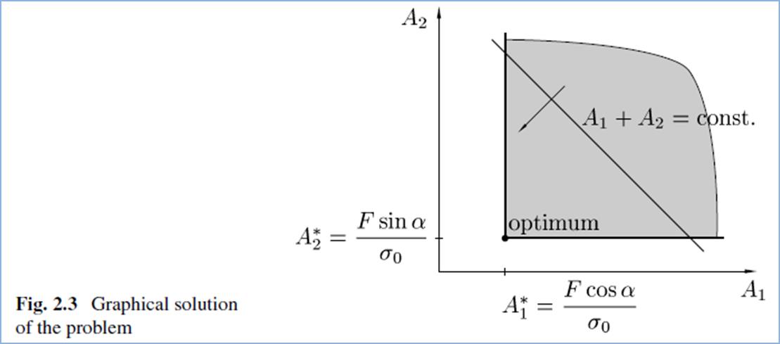
Figure 2‑6 - A graphical representation of a simple
two bar optimisation problem showing the limiting conditions reproduced from (Christensen PW, 2008)
Unfortunately, as the structural systems analysed become
more complex the optimisation functions get increasingly difficult to plot, and
the problems become multi-dimensional. Also it is very difficult to form
optimisation functions for arbitrary structures.
An older publication (Haftka & Grandhi, 1986) provides
an overview of shape optimisation techniques and a similar publication (Topping, 1983) provides a similar overview for skeletal structures. These divide
structural optimisation criteria into size optimisation, topology optimisation
and shape optimisation problems. Size optimisation problems seek to minimise section
sizes whilst maintaining the fixed geometry (as applicable to this project).
Topology optimisation methods generally reduce the number of elements whilst
staying within the prescribed optimisation criteria. Finally, shape
optimisation algorithms alter the coordinates of nodes. The latter two do not
apply to this project.
Figure 2‑7 Graphical representation of a typical shape
and topology optimisation problem reproduced from (Venetsanos, 2010)
Based on the similar original principles, the structural
optimisation methods have been developed since aided by new research as well as
the advances in computer technology allowing for more powerful and complicated
algorithms to be implemented. The (Venetsanos, 2010) PhD thesis provides a very
extensive overview of current research on the topic. The paper acknowledges
that the three optimisation methods listed above cannot be easily decoupled and
that modern approaches generally adopt a combination of methods with the newer
research heavily concentrating on developing shape and topology optimisation
procedures.
Another good and recent publication offering extensive
information on the topic is (Spillers & MacBain, 2009). It goes into great
detail into Sequential Linear Programming and the Incremental Equations of
Structures techniques. These are currently most widely used and researched
techniques in structural optimisation. Linear programming
relies on setting up the problem as a series of linear objective functions
subject to linear equality or inequality constraints forming the feasible
region - a convex polyhedrona. A suitable linear programming algorithm is then
used to find a point a point in the polyhedron where this function has the
smallest (or largest) value if such a point exists (Wikipedia, 2013).
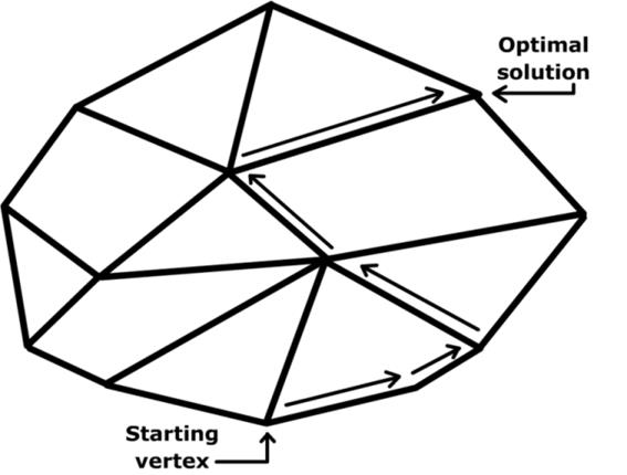
Figure 2‑8 A diagram demonstrating how a Simplex
Algorithm is utilised to demonstrate how the optimum solution is found within
the polytope
There are numerous mathematical methods developed for
optimisation in general. Some are more suitable than others for application
than others in the field of structural optimisation. Some of the particular
issues include the necessity to utilise the available section sizes, meaning
that the potential solution is discretised and not continuous. If using
continuous criteria, selecting the closest available selection alters the
stiffness matrix from that analysed and can either lead to non-optimal or even
non-stable solution. Hence, most structural optimisation techniques rely on
iterative approach to a learn7-programming-finite-elements-in-javascript.htm. Also, because there is normally an infinite
number of solutions there is a real risk that the optimisation algorithm will
reach a local minima, rather than an absolute one. Therefore, the recent
advances have relied on introducing the learn7-programming-finite-elements-in-javascript.htm of randomness (similar to
mutations in the evolution theory) to ensure that a number of varied solutions
are tested in an attempt to truly reach a global optimal solution.
Many of the research papers looking at current developments
in Structural Optimisation are printed within the Journal of
Structural and Multidisciplinary Optimisation, such as (Mela & Koski, 2012), (Le Riche & Haftka, 2012), and also within other scientific
publications (Croce, et al., n.d.) (Talaslioglu, 2009) and many others.
The iterative approach utilised in development of the
application is not grossly dissimilar to the approach presented by (Guerlement, et al., 2001). The procedure presented in the paper attempts to find the
optimal solution by starting from the heaviest section available and reduces
the section to the minimal section that passes ULS and SLS checks. The
procedure implemented within the application works in the opposite direction by
starting with the smallest available section (for the selected type) and then
upgrades the section sizes until all sections meet SLS and ULS criteria. The
approach is further detailed below.
Background Information
When sizing each element, a structural engineer normally
attempts to select the smallest section that meets the Ultimate Limit State
(strength) and the Serviceability
Limit State criteria. An iterative
technique is often used by engineers to find the optimal solution, whereby
an initial section is assumed based on experience and then checked by
calculations. If the structural checks fail, the engineer selects a bigger
section. On the other hand, if the utilisation of the section is small, the
engineer may attempt to justify the use of a smaller section in order to
optimise the solution. This is generally a long-winded process and relies on
the experience of the engineer to select the initial section and the time
constraints required to carry out the necessary iterations.
Outside engineering, optimisation techniques have mostly
developed as a part of management studies with the aim of optimising production
within a company in order to utilise the company’s resources in the most
effective way and maximise profits. Management optimisation techniques
generally attempt to define a problem as a set of mathematical functions,
introduce optimisation limits and criteria, and then use mathematical methods
to find the optimal solution(s). There are numerous textbooks dealing with this
topic as a general problem.
The procedure employed in developing the application uses an
approach somewhat similar to the iterative procedure carried out by manual
calculations rather than attempting to define the problem mathematically. It
relies on the great computational power offered by modern computers.
Optimisation tool in konstrct.com
Whilst it is relatively simple to define an optimisation
problem and set up the relevant criteria for specific optimisation problems, it
is significantly more difficult to successfully set-up a broad procedure that
will work for any (or most) of the assemblies that a user of an application can
input.
To illustrate the issue, a simple portal frame problem is
presented – an almost infinite number of solutions exist for this problem to
include strong column-weak rafter, balanced column-rafter and weak
column-strong rafter. Optimising for any route produces local optima, but any
of these can be a true global optimal solution. It would not be practical to
analyse every possible solution. Finally, changing any of the member properties
alters the structure stiffness matrix, and thus the distribution of member
forces, and the full analysis must be rerun for every possible case.
As the scope of the project is very broad, a relatively simple
iterative technique was adopted. The analysis is initially run with the
smallest available section for a chosen section type. Each section is then
upgraded to the minimum section that passes ULS checks. The procedure then
reruns analysis with the upgraded sections and updated stiffness matrix and
reruns all ULS checks and further upgrades sections as necessary. SLS Checks
are carried out only if all sections pass ULS checks. This is repeated until
all sections pass ULS and SLS checks. The algorithm can optimise each element
for minimum weight or minimum section height. A simplified flow diagram of the
algorithm is included overleaf to illustrate the procedure.
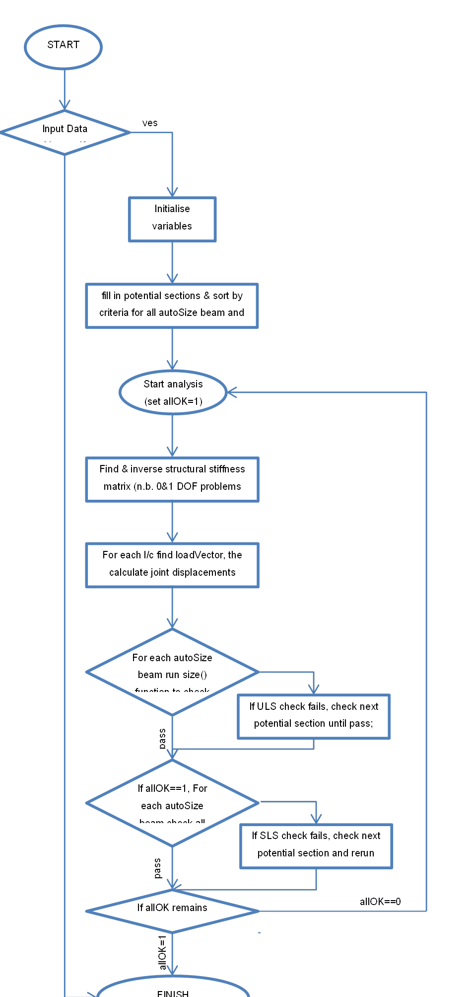
Figure 4‑1 - Outline optimise() function flow diagram
A full EC3 code check is carried out for each ULS check,
whereas SLS checks that deflections at any point of the beam do not exceed the
prescribed limit. To speed up processing time, simplified capacity checks have
been introduced to the ULS sizing algorithm to quickly discard sections that
fail simple capacity checks (M/W*py>1.1, N/A*py>1.1, etc), and only
perform full checks for sections that are likely to pass.
This approach leads to a fairly balanced result (e.g. in an
example of a simple portal frame, leads to similarly sized rafter and column).
This returns one of the local minima but for problems with a high learn7-programming-finite-elements-in-javascript.htm of
static indeterminacy may not lead to the actual optimal solution. Also the
procedure is very resource intensive as it involves carrying out multiple
comprehensive EC3 sizing checks which may include Buckling and Lateral
Torsional Buckling checks. However, for small assemblies, results are normally
presented within a few seconds on a mid-range PC. For structurally determinate
systems, and for many indeterminate systems the returned solution is globally
optimal.
There is a number of other criteria other than section
weight that should be met to truly design the most cost-effective structure.
This includes minimising the number of different sections to be used (and thus
minimise wastage) or minimising the number of joints (as these are labour
intensive and thus expensive). These cannot be simply be implemented within an
automated sizing criteria, and a learn7-programming-finite-elements-in-javascript.htm of engineering judgement still remains
crucial.
A competent and experienced engineer can and should exercise
his engineering judgement to fix the size of certain elements after the initial
run to address the criteria above. For example, in order to obtain a truly
optimal solution for a portal frame problem presented previously; the engineer
can fix an oversized column section and let the algorithm select the matching
rafter section. By manually iterating only a few column sections, the engineer
should be able to obtain the truly optimal solution for a portal frame.
Obviously, extending the structural analysis module to handle non-linear
effects would further improve the results!
Programming Structural Analysis and Finite Elements in JavaScript
Javascript
is an object-based and prototype-based language, and as such the application
code is split into various objects containing their properties and methods. This
is different to many higher level languages such as Java or C which are
class-based.
beam Object (properties)
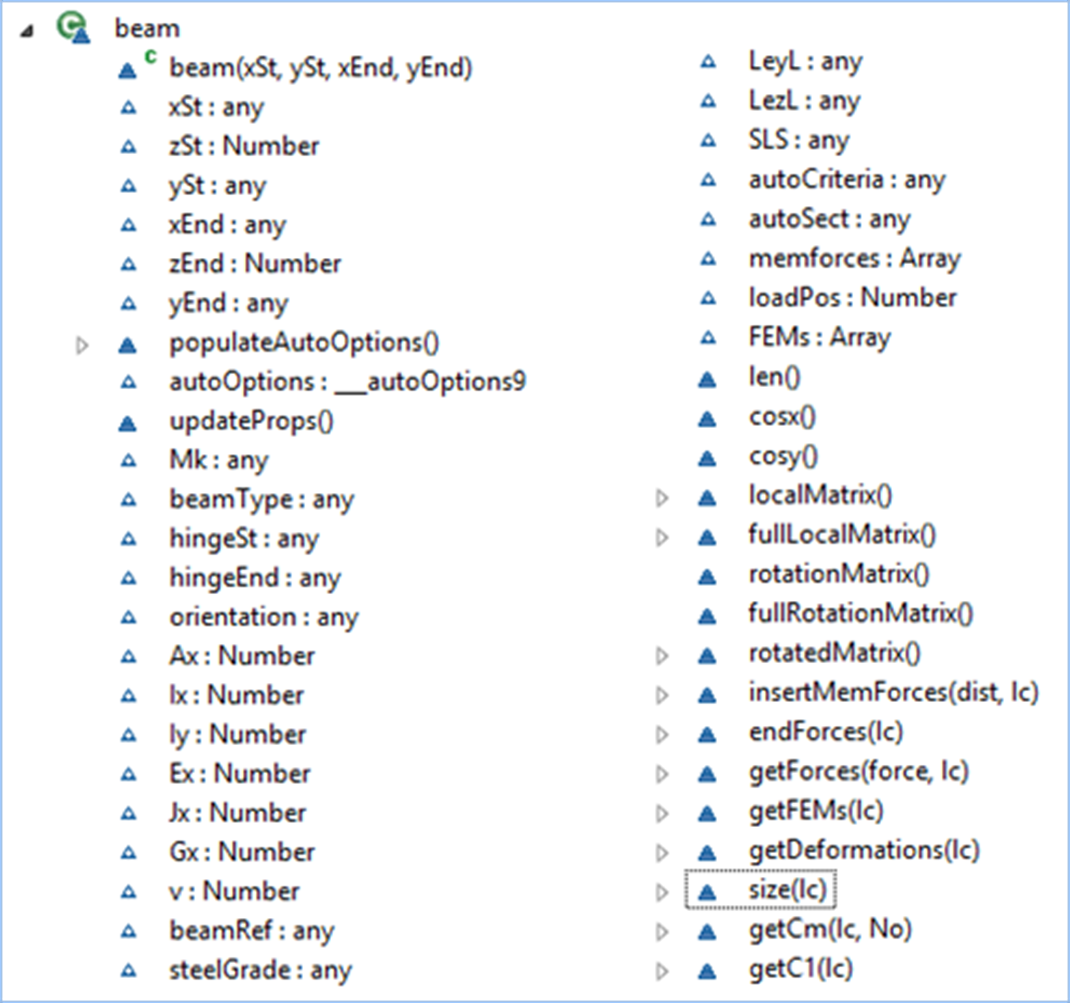
Figure 3‑1 Beam Object UML Diagram Showing Available
Properties and Methods
All instances of beam objects are contained within the
beams() array.
Beam object has the following properties:
- xSt,
ySt, zSt, xEnd, yEnd, zEnd – start and end coordinates, where zSt and zEnd are
fixed at 0 for 2D problems.
- Mk
– Beam Mark (reference)
- beamType
– Type of beam – e.g. "generic", "Steel Section" or "Auto
Steel" corresponding to different types of beams that can be inputted.
Obviously this can be expanded in the future to include standard materials
(steel/concrete/timber) and some standard sections where section properties can
be easily calculated (e.g. rectangular, circular, hollow box or circular
sections, etc).
- hingeSt
and hingeEnd – have a value of 1 or 0 depending on whether a hinge at the end
of the beam is present or not.
- orientation
- Orientation of the beam – has a value of 0 if the major axis of the beam
lies in-plane (plane frames) or a value of 1 if it is perpendicular to the
plane (grillages)
There are further specific properties for different section
types. For generic sections, values of A, Ix, Iy, E, J, G and v are inputted
manually.
beam Object procedures and functions
Beam is the most complicated object and contains nearly 1/3
of the code of the entire application (1500+ lines of code). It contains a
large number of methods that are generally represented by functions and return
an appropriate result. All beam methods are listed below. Some are very simple,
and their names are generally self-explanatory, whereas the more complex
methods will be described in more detail.
this.updateProps - updates member properties from defaults
values - normally used whenever a beam object is created.
this.memforces - contains free bending moment diagram and
other member forces for a simply-supported member and calculated by the
loadVector() function for all member loads during analysis. These are normally
modified by the this.getForces function to produce member forces adjusted for
fixed-end forces taken from the analysis
this.len - returns the length of the member
this.cosx, this.cosy - returns direction cosines about the x
and y axes (direction cosine about the y axis = direction sine about the x axis)
this.fullLocalMatrix - returns a member matrix for a 3D
element. Calculates all stiffness coefficients and returns a matrix object. The
matrix is adjusted for hinges and also Ix and Iy are inverted for members that
are treated as grillage elements (i.e. major axis of a member perpendicular to
the x-y plane). A typical matrix for a bar element with no hinges is as follows:
E*A/L
border-left:none;padding:0cm 2.85pt 0cm 2.85pt;height:1.0pt'>
border-left:none;padding:0cm 2.85pt 0cm 2.85pt;height:1.0pt'>
border-left:none;padding:0cm 2.85pt 0cm 2.85pt;height:1.0pt'>
border-left:none;padding:0cm 2.85pt 0cm 2.85pt;height:1.0pt'>
border-left:none;padding:0cm 2.85pt 0cm 2.85pt;height:1.0pt'>
border-left:none;padding:0cm 2.85pt 0cm 2.85pt;height:1.0pt'>
-1*E*A/L
border-left:none;padding:0cm 2.85pt 0cm 2.85pt;height:1.0pt'>
border-left:none;padding:0cm 2.85pt 0cm 2.85pt;height:1.0pt'>
border-left:none;padding:0cm 2.85pt 0cm 2.85pt;height:1.0pt'>
border-left:none;padding:0cm 2.85pt 0cm 2.85pt;height:1.0pt'>
border-left:none;padding:0cm 2.85pt 0cm 2.85pt;height:1.0pt'>
12*E*Ix /L/L/L
6*E*Ix /L/L
-12*E*Ix /L/L/L
6*E*Ix /L/L
12*E*Iy /L/L/L
-6*E*Iy /L/L
-12*E*Iy /L/L/L
-6*E*Iy /L/L
G*J/L
-1*G*J/L
-6*E*Iy /L/L
4*E*Iy/L
6*E*Iy /L/L
2*E*Iy/L
6*E*Ix /L/L
4*E*Ix/L
-6*E*Ix /L/L
2*E*Ix/L
-1*E*A/L
E*A/L
-12*E*Ix /L/L/L
-6*E*Ix /L/L
12*E*Ix /L/L/L
-6*E*Ix /L/L
-12*E*Iy /L/L/L
6*E*Iy /L/L
12*E*Iy /L/L/L
6*E*Iy /L/L
-1*J*G/L
J*G/L
-6*E*Iy /L/L
2*E*Iy/L
6*E*Iy /L/L
4*E*Iy/L
6*E*Ix /L/L
2*E*Ix/L
-6*E*Ix /L/L
4*E*Ix/L
Table 3‑1 - Element Stiffness Matrix
this.fullRotationMatrix - returns a 3D rotation matrix for
an element and use for the rotation of the element
stiffness matrix and for coordinate transformations. All member loading
needs to be converted from ‘Local’ or ‘Member’ coordinate system
into ‘Global’ coordinate system to form a solution. Similarly, to obtain
member forces, the global resulting displacement and member forces are
transformed and outputted in Local member coordinates. All angle displacements
and moments remain unchanged; whereas vertical and horizontal forces and
displacements are multiplied by the sine or cosine of the angle of the
inclination of the member α (Transformations are achieved through the
application of the principle of contragredience (Jenkins, 1969)).
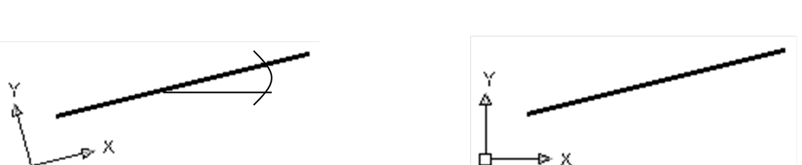
Table 3‑2 Graphical Presentation of Coordinate
Transformation
this.endForces(lc) - returns member end forces for an
inputed load case.
this.getForces = function(force,lc) - returns an array
containing moments along the length of the beam, where force=0:axial;1:shears
x-x;2:shear y-y; 3:torsion; 4:moments y-y; 5:moments x-x 6:lengths along
this.getDeformations(lc) - returns
deformations in all three directions in local member axes. For the inputted
loadcase, calculate and sum two components of deflections. The first component
obtained by interpolating the end displacements and rotations using the
appropriate shape function:
This is based on the information provided within the lecture
notes by (Chandra & Namilae, n.d.)
The second component of deflection was originally calculated
by integrating the bending moment diagram for an equivalent en-castre member
(moment-area theorem) - based on the guidance provided within (Prakash, 1997).
The procedure is carried out twice for both in-plane and
out-of-plane deformations and with making allowance for hinged member where
appropriate. Because the end-rotation for hinged members cannot be extracted
from the displacement matrix directly (as it equals 0 for hinged members), it
will need to be calculated when the loadVector is formed. This functionality is
yet to be implemented, thus the displacements for hinged members are currently
incorrect.
This method has proven difficult to implement for hinged
members. Thus a simpler approach of directly calculating member deflections
using formulae by the loadvector() function available at http://www.tquigley.com/T312.htm
was adopted for the final version.
support Object
Figure 3‑8 Support Object UML Diagram Showing the
Available Properties and Methods
The support object is far less complex than the beam object,
and it only contains support coordinates and values of 0 or 1 for each of the
restraint conditions.
updateProps() method is invoked when a support object is
created to fill in default restraint values.
pLoad Object
Figure 3‑9 pLoad object - Showing the Available Properties
and Methods
pLoad object is not dissimilar to the support object, and
only contain properties of inputted point loads. These include load coordinates
and intensity as well as the assigned load case (lc).
lLoad Object
Figure 3‑10 lLoad Object UML Diagram Showing the
Available Properties and Methods
lLoad object contains line load start and end coordinates,
start and end intensities and the load case.
updateProps() method updates object properties and len()
returns the length of the line load.
Structural Analysis
Structural analysis is performed by a series of functions.
The code was subdivided into individual functions to simplify debugging and to
be able to call up parts of the procedure as required. The analysis utilises
the standard stiffness method, and the implementation is loosely based on the
Matrix Structural Analysis of Plane Frames using Scilab (Annigeri S, 2009). The
publication, which forms a part of Prof Annigeri‘s lecture notes provides
extensive guidance on forming the relevant matrices and extracting member
forces, and also provides examples which allow for quick verification of the
code. The algorithm was adopted for the use in JavaScript with Sylveter Matrix
library, and to allow for additional learn7-programming-finite-elements-in-javascript.htms of freedom, hinges, member loads
etc. All matrix
manipulations were handled by the JavaScript
Matrix library Sylvester developed by JC Coglan. The library and API
documentation is available at (Coglan, 2007-2012) and handles matrix
manipulations such as multiplication, inversion etc.
getNodes function loops all beams and assigns nodes then
stores node coordinates and stores them within the nodes() array. In order to
establish connectivity between members, each potential new node is checked
against the existing array to avoid creating duplicates.
Function locationMatrix() forms the
location matrix and calculates the number of learn7-programming-finite-elements-in-javascript.htms of freedom (ndof). It
loops all nodes and for each learn7-programming-finite-elements-in-javascript.htm of freedom that is not restrained assigns a
consecutive integer within the location matrix. All restrained nodes are
assigned a zero within the location matrix. Rows within the matrix correspond
to nodes, and columns to learn7-programming-finite-elements-in-javascript.htms of freedom. Thus a typical location matrix for
a simply supported beam would be:
[0, 0, 0, 0, 1, 2]
[0, 3, 0, 0, 4, 5]
Note that the structural analysis algorithm allows for potentially 6 learn7-programming-finite-elements-in-javascript.htms of
freedom at each node: x-axis translation, y-axis translation, z-axis
translation (out of plane), torsional rotation, out of plane rotation and
in-plane rotation. This allows for analysis of both plane frames and grillages.
structureSMatrix() function calls up the beam.rotatedMatrix()
function for each of the beams (please see previous section) which returns the
rotated stiffness matrix and then sums up the appropriate stiffness coefficients
to form the structure stiffness matrix. The references to rows and columns
within the matrix correspond to integers within the locationMatrix(), and all
restrained DOFs are eliminated from the structure stiffness matrix to allow for
supports and also to reduce computational workload associated with manipulating
the structure stiffness matrix. The function returns a Sylvester matrix object
to allow for further manipulation.
loadVector(lc) function is complex as it
forms the load vector for any given loadcase, but also stores the relevant
free member force diagrams (e.g. free BM diagram), end displacements that are
used for displaying member force results. The function loops through all joint
loads and then also discretises all line loads into a series of individual
point loads (between 41 and 99 depending on the relative length of the line
load and the minimum beam length). This forms an allLoads() array. loadVector()
function then loops through all loads to find loads applied at nodes. These are
immediately inserted into the loadVector array. All loads applied directly on a
supported node corresponding directly to the supported DOF are directly saved
within the reactions() array and are disregarded from further analysis
Member loads require significantly more attention. Firstly,
all loads are rotated into member coordinate system and split into a component
perpendicular to the beam and a component along the beam. Out-of-plane loads do
not require rotating as these are always perpendicular to the x-y plane (for
grillages). The algorithm then calculates the end forces and inserts them into
the loadVector. It also calculates free member forces and stores them in
beam.memforces for each beam and for each loadcase. The effects of all point
loads (or discretised line loads) are summed. Allowance for hinges is also made
as required. The algorithm also stores whether all loads are applied within the
central ¼ of the beam length so as to be able to select the appropriate Lateral
Torsional Buckling coefficients in the sizing algorithm. The function returns a
Sylvester matrix object to allow for further manipulation. Because Sylvester
library does not work with 0 and 1 element matrices (corresponding to 0 or 1
DOFs), these are treated differently.
Graphical Display and Interaction – Canvas
There are two main ways of displaying and interaction with
graphical information on the web currently – Scalable Vector Graphics (SVG) and
the Canvas element. Whilst both have their advantages and disadvantages, canvas
is a more recent development and has significant performance advantages when
dealing with a large number of graphical elements. Generally, SVG keeps
graphics in vector format and assigns a DOM reference to each of the new
elements, which consumes a lot of RAM and processor resources, but makes it
much easier to interact with.
The Canvas HTML element, as its name states, acts as a
simple drawing canvas where the graphical information is to be displayed. Once
an object is drawn onto the canvas it cannot be addressed any more. This
reduces the memory footprint for difficult scenes, but it makes it somewhat
more difficult to interact with.
The canvas features its own coordinate system which can be
translated, rotated and scaled to suit.
As it is difficult to alter the contents of the canvas, the
normal approach is to redraw the canvas whenever the contents changes. This is
handled by the redraw() function and normally takes a small fraction of a
second. In games, the canvas is usually redrawn 30 or 60 times per second to
maintain fluid animation, but this approach is not necessary with this interactive
application.
When displaying the main structural elements, the canvas
coordinate system is normally scaled and panned so that it matches the global
structure coordinate system. The draw coordinates are thus inputted in the
global coordinates. On the other hand, when displaying member forces and
deformations, the Canvas coordinate system is rotated, translated and scaled to
match the local coordinate system of each beam and the forces are plotted
directly. Thus, all complex coordinate transformations are handled by the
JavaScript engine which runs on native code and is highly optimised and far
quicker to execute. It also avoids the need to manually transform coordinates.
At the moment, for input, all clicks are snapped to a major
or a minor grid (if either is toggled on), or can be freely clicked. For future
development, the UI should be expanded to allow numerical input of coordinates
(relative and absolute) and snapping to intersection, end and mid points
similar to CAD applications. It is also possible to import member geometry from
a DXF file (which can be exported from CAD applications). Imported geometry is
snapped to the 0.1m grid by default.
Because the elements are not identified directly, an
elaborate technique of using a shadow canvas (a second canvas that is not
displayed and only exists in memory) is created to match the main canvas in
size. Each of the elements is then plotted onto the shadow canvas and the colour
of the clicked pixel is queried until a match is found. This is one of the many
techniques used for detecting selections on a canvas and is very versatile as
it does not require the clicks to be identified from element geometry and
enables the detection of complex objects. The technique is described in detail
in the
Gentle Introduction to Making HTML5 Canvas Interactive (Sarris, 2011). Detecting double-clicks uses the same technique and facilitates the deletion of
elements.
Bibliography
Annigeri S, P., 2009. Matrix Structural Analysis of
Plane Frames. Hubli: Department of Civil Engineering.
Brettle, M. E., 2009. Steel Building Design: Worked
Examples - Open sections. Ascot, UK: The Steel Construction Institute.
Brettle, M. E. & Brown, D. G., 2008. Steel
Building Design: Worked Examples - Hollow Sections. Ascot: The Steel
Construction Institute. .
Brettle, M. E. & Brown, D. G., 2009. Steel
Building Design: Concise Eurocodes.. Ascot: The Steel Construction Institute.
Bureau, A. & Galea, Y., 2010. NCCI: Elastic
critical moment for lateral torsional buckling, NCCI Access Steel Document
SN003b-EN-EU, s.l.: Access Steel.
CEN, 2005. EN 1993-1-1: General rules and rules for
buildings for the design of steel structures, s.l.: CEN, BSi.
Chandra, N. & Namilae, S., n.d. Lecture notes
for module Design Using FEM (EML4536 / EML5537). [Online]
Available at: http://www.eng.fsu.edu/~chandra/courses/eml4536/
[Accessed May 2013].
Christensen PW, K. A., 2008. An introduction to structural
optimisation. Linköping: Springer.
Coates, R. T., Coutie, M. G. & Kong, F. K., 1987. Structural
Analysis. 3rd ed. Wokingham, UK: Van Nostrand Reinhold (UK).
Coglan, J., 2007-2012. Sylvester JavaScript Library
API Document. [Online]
Available at: http://sylvester.jcoglan.com/
[Accessed 2012 5 3].
Croce, E. S., Ferreira, E. G. & Lemonge, A. C. C.,
n.d. A GENETIC ALGORITHM FOR STRUCTURAL OPTIMIZATION OF STEEL, s.l.:
s.n.
E, B. M. & Brown, D. G., 2009. Steel Building
Design: Worked Examples - Open Sections. Ascot: The Steel Construction
Institute.
Felippa, C. A., 2000. A Historical Outline of
Matrix Structural Analysis:, Boulder, USA: University of Colorado.
Felippa, C. A., 2004. Introduction to FEM, Chapter
12, Variational Formulation of Plane Beam Element, Boulder, Colorado, USA:
University of Colorado.
Fulton, S. & Fulton, J., 2011. HTML5 Canvas. 1st
ed. Sebastopol, USA: O'Riley.
Gavin, H. P., 2009. CE 131L. Matrix Structural
Analysis - 3-D TRUSS ANALYSIS. s.l.:Duke University, Department of Civil
and Environmental Engineering.
Guerlement, G. et al., 2001. Discrete minimum weight
design of steel structures using EC3. Struct Multidisc Optim 22, p.
322–327.
Haftka, R. & Grandhi, R., 1986. Structural Shape
Otpimisation - A survey. Computer Methods in Applied Mechanics and
Engineering , Issue 57, pp. 91-106.
Hawkes, R., 2011. Foundation HTML5 Canvas for Games
and Entertainment. Bournemouth, UK: friendsofed, Apres.
Jenkins, W., 1969. Matrix and Digital Computer
Methods in Structural Analysis. s.l.:McGraw-Hill.
jointly published by the The Steel Construction
Institute, Tata Steel & The British Constructional Steelwork Association
Ltd., 2011. Steel Building Design: Design Data. s.l.:s.n.
Le Riche, R. & Haftka, R. T., 2012. On global
optimization articles in SMO. Structural and Multidisciplinary Optimization,
Volume 46, p. 627–629.
McFarland, D. S., 2011. JavaScript & jQuert:
The Missing Manual. Portland, Oregon, USA: O'Reily.
Mela, K. & Koski, J., 2012. On the equivalence of
minimum compliance. Structural and Multidisciplinary Optimization, Volume
46, p. 679–691.
Nikishkov, G., 2010. Programming Finite Elements in
Java. Aizu, Japan: Springer.
Pilgrim, M., n.d. Dive Into HTML5. [Online]
Available at: http://diveintohtml5.info/
[Accessed 7 7 2013].
Prakash, R., 1997. Graphical Methods in Structural
Analysis. Hyderguda, India: Universities Press.
Sagaseta, J., 2012. Lecture Notes for module
ENGM053 - Structural Mechanics and Finite Elements. Guilford, UK: Surrey
University.
Sarris, S., 2011. A Gentle Introduction to Making
HTML5 Canvas Interactive. [Online]
Available at: http://simonsarris.com/blog/510-making-html5-canvas-useful
[Accessed 7 7 2013].
Simpson, K., 2012. JavaScript and HTML5 Now. s.l.:O'Reilly
Media.
Spillers, W. R. & MacBain, K. M., 2009. Structural
Optimization. New Jersey, USA: Springer.
Talaslioglu, T., 2009. A New Genetic Algorithm
Methodology for Design Optimization of Truss Structures: Bipopulation-Based
Genetic Algorithm with Enhanced Interval Search. Modelling and Simulation in
Engineering, Volume 2009, p. 28.
Tata Steel, n.d. The new interactive bluebook. [Online]
Available at: http://tsbluebook.steel-sci.org/default.htm
Topping, B., 1983. Shape Optimization of Skeletal
Structures: A Review. Struct. Eng, Volume 109(8), p. 1933–1951.
Venetsanos, D. T., 2010. Development Of Methods For
Topology And Shape Optimization Of Mechanical Structures. Athens, Greece:
s.n.
Wikipedia, 2013. Linear Programming. [Online]
Available at: http://en.wikipedia.org/wiki/Linear_programming
[Accessed 8 2013].
Wikipedia, 2013. List of finite element software
packages. [Online]
Available at: http://en.wikipedia.org/wiki/List_of_finite_element_software_packages
[Accessed August 2013].
Wikipedia, n.d. [Online]
Available at: http://en.wikipedia.org/wiki/Structural_analysis
[Accessed 2014].
Wikipedia, n.d. HTML5. [Online]
Available at: http://en.wikipedia.org/wiki/HTML5
[Accessed 7 7 2013].
Wikipedia, n.d. Java (programming language). [Online]
Available at: http://en.wikipedia.org/wiki/Java_%28programming_language%29
[Accessed 12/09/2011].
Wilton, P. & McPeak, J., 2010. Beginning
JavaScript. Indianapolis, USA: Wiley.
Zienkiewicz, O. C. & Taylor, R. L., 2000. The
Finite Element Method, Volume 1. 5th ed. Oxford, UK: Butterworth Heinmann.
Konstrct.com is a fully web-based structural analysis tool built using web-technologies incuding JavaScript and html5. It can be used to perform structural analysis of plane frames and grillages, and automated steel sizing and optimisation to Eurocode 3 (EC3).
The application runs within a web browser and are thus fully portable and compatible with a large variety of devices such a smartphones, tablets and PCs. This is in contrast to most structural analysis tools in use today which are often very feature rich and efficient, but remain mostly PC based.
The application was developed over a period of some three years and build upon an MSc project in Structural Engineering at the University of Surrey.
The structural analysis utilises the stiffness method and the application contains an optimisation tool is based on an iterative technique to select the optimal steel sections based on the prescribed criteria (minimum weight or section height).
The graphical user interface is fully html5 and standards based and the graphical display and interaction was built using the recently introduced canvas element.
Because it is standards based, the application was successfully tested on many different platforms including different PC browsers (Mozilla, Chrome, IE), tablets (iOS and Android) and also smart phones (iPhone and Android).
Current Limitations and Future Work
The application remains in beta, and more testing is required to validate many different scenarios that can be analysed.
The application is currently limited to beam elements only and only allows for linear analysis. The addition of non-linear analysis and other types of elements which would enable the analysis of slabs and shells is expected to be introduced in the future.
Whilst functional, the optimisation algorithm remains somewhat basic, and will not produce a true optimal solution for problems with a high learn7-programming-finite-elements-in-javascript.htm of static indeterminacy. In such cases it is likely that the algorithm will lead towards a local minima rather than a true global optimum as discussed in the Optimisation section.
By using this software you agree to the terms and conditions
below
THE SOFTWARE IS PROVIDED 'AS IS', WITHOUT WARRANTY OF ANY KIND, EXPRESS
OR IMPLIED, INCLUDING BUT NOT LIMITED TO THE WARRANTIES OF MERCHANTABILITY, FITNESS
FOR A PARTICULAR PURPOSE AND NONINFRINGEMENT. IN NO EVENT SHALL THE AUTHORS OR
COPYRIGHT HOLDERS BE LIABLE FOR ANY CLAIM, DAMAGES OR OTHER LIABILITY, WHETHER
IN AN ACTION OF CONTRACT, TORT OR OTHERWISE, ARISING FROM, OUT OF OR IN
CONNECTION WITH THE SOFTWARE OR THE USE OR OTHER DEALINGS IN THE SOFTWARE.
User Interface – Manual
This application is still in development - use with caution!
Structural software is not a replacement for the knowledge of structural
design.
The application should only be used by a trained, qualified and experienced
engineer or for learning and training. All results must be checked by hand
calculations!
Structural Analysis EC3 Sizing+Optimisation Application for html5 and
JavaScript
Copyright (c) 2011-2014 Marko Nesovic, all rights reserved
Brief Instructions:
-You need at least some beams, some supports and some loads to run analysis
-To delete elements, double-click on them
-To improve performance use few auto-size members and fix the size of as many
beams
as possible by changing their type from auto to steel section
If you have any comments, please contact me on konstrct (at) outlook . com
By using this software you agree to the terms and conditions below
THE SOFTWARE IS PROVIDED 'AS IS', WITHOUT WARRANTY OF ANY KIND, EXPRESS
OR IMPLIED, INCLUDING BUT NOT LIMITED TO THE WARRANTIES OF MERCHANTABILITY,
FITNESS FOR A PARTICULAR PURPOSE AND NONINFRINGEMENT. IN NO EVENT SHALL THE
AUTHORS OR COPYRIGHT HOLDERS BE LIABLE FOR ANY CLAIM, DAMAGES OR OTHER
LIABILITY, WHETHER IN AN ACTION OF CONTRACT, TORT OR OTHERWISE, ARISING FROM,
OUT OF OR IN CONNECTION WITH THE SOFTWARE OR THE USE OR OTHER DEALINGS IN THE
SOFTWARE.
The user interface enables rapid development, testing and validation of the application. The UI enables graphical input of data (beams, supports and loading) as well as the graphical output of results.
The user interface is fully HTML5 based and include standard HTML elements, whereas a canvas graphical element (new to HTML5) is used for the display of graphical information and for graphic input. Interactivity is provided through JavaScript, which provides both interaction with forms and buttons as well as drawing within the canvas element and interactivity within the canvas. Konstrct.com utilises twitter bootstrap to improve the visual quality of the application and provide the necessary scalability for various screen sizes.
Visually, the aim was to keep the layout as simple as possible whilst providing all the required functionality. This was done so that the application does not appear cluttered and daunting to potential novice users but still enabling access to finer levels of input and accurate structural modelling and sensible sizing of structural elements.
The UI was structured to enable the application to be used both on a PC with keyboard and a mouse and on touchscreen phones and tables (iOS or Android based). It was tested in Mozilla Firefox, Chrome and Internet Explorer (later versions enabling HMTL5 support). No major incompatibilities between different systems were encountered.
As with most structural analysis applications, the UI is split into two main elements – input of data and output of results. The main input screen enables the user to select elements (in order to edit their properties) or delete them by double-clicking or double-tapping. It also enables the user to input the general information about the project such as name, ref number etc.
Figure 3‑11 - Main input screen
The structural elements available for input include beams, supports, line and point loads. All are inputted graphically by clicking on the main drawing canvas. By default a 1m major grid is enabled and all clicks are snapped to it. It is possible to turn it off and a 0.1m minor grid is also available for higher precision. The canvas can be zoomed in and panned. Using the minor and major grid as well as zooming and panning, it is possible to easily input and model various structural problems with 0.1m accuracy either on a PC or on touch-screen devices.
Numerical data/properties are inputted through a table/form displayed on the right hand side of the screen. The contents of the form changes to suit the currently selected element. Also, for beams, the form changes to accommodate different types of input required for defining different types of beams. Please see the forms reproduced below.
Figure 3‑12 Supports and Loading Input Forms
Figure 3‑13 Beam Data Input Forms
The application provides the following output:
- a. AxialForces
- b. Shear Forces (in-plane)
- c. Shear Forces (out-of-plane)
- d. Bending Moments (in-plane)
- e. Bending Moments (out-of-plane)
- f. Torsion
- g. Deformations (in-plane)
- h. Deformations (out-of-plane)
- i. Reactions
- j. Matrices:
- i. Structure Stiffness Matrix
- ii. Location Matrix
- iii. Load Vector
- iv. Member Matrices
- v.Global Displacement Matrix
- vi. Member End Forces
- k. Member Sizing
A single screenshot is presented below showing a typical bending moment diagram for a portal frame subject to a point load at mid-span.
Figure 3‑14 Typical Output Diagram (BM diagram)
Treatment of frames and grillages
The main plane of the screen is treated as an x-y plane, and the z axis is taken to be perpendicular to it. Loading can be inputted in all three axis and results can be obtained in-plane and out-of plane. This enables the analysis of both plane frames and grillages depending on how data is inputted.
If loads are only inputted in the x and y axes, then the problem is a plane analysis case, and the user should only seek in-plane results. On the other hand, if loading is inputted in the z-axis, then the user should look at out-of-plane member forces. Obviously, it is possible to combine both and get results in both directions to analyse, for example, a frame subject to both vertical (gravity) and out-of-plane lateral loading (e.g. wind).
A switch within the beams input form allows the user to set the orientation of the beam, or more precisely, select whether the major axis of a beam sits in-plane or out-of-plane.
Structural Analysis Software and Methods
Structural analysis tools have been created ever since the development of early computers because these allow for rapid solution of complicated structural problems in the fraction of the time required to do hand calculations. The initial tools were very basic in both functionality and performance offered by the computers in the past. However, over time, comprehensive software was developed, and modern structural applications now offer full analysis, design and optimisation solutions helping engineers rapidly prepare designs of very complex structures. The advances in structural analysis now enable engineers to analyse structures that even 15 years ago would not have been possible to model and design accurately. Most of the existing tools were developed in low-level languages such as Java or C++ and remain PC based.
When looking at the literature on computer based structural analysis and the stiffness method a lot of guidance and code is available in Fortran, Basic, C and Java. Software developed using these programming languages is tied to the hardware and the operating system that it has been compiled and developed for and porting such applications to different platforms is often very difficult.
A good number of Java based structural analysis tools have also been developed in the past and some books have been published on the topic. Whilst significantly more portable, Java applications require that a Java Virtual Machine (JVM) be installed on the computer to be able to run which can be cumbersome, and many user choose not to (or don’t know how to) have it installed. There is a wealth of information on programming structural analysis software in Java, and a book Programming Finite Elements in Java (Nikishkov, 2010) provides extensive guidance. Some of the chapters from this book can be applied to this project.
There are many structural analysis (and design) packages available on the market. Unlike many markets where individual players have managed to achieve very large market share, and set their software as de-facto industry standards, the market for structural analysis software is still very much fragmented with many options available. In addition, many larger practices still maintain and develop their in-house structural software.
Most of the original software developed in the 80s was very basic, had non-existent or very basic graphical output and often only textual data input and included a very limited array of elements. The 90s saw the development of full graphical interfaces that allowed for much easier modelling of structures. The functionality of software was expanded to include non-linear analysis, flexible supports, movable loads, load combinations, etc. The software popular at the time included SAAP, STAD and many others.
In the past 10 years, the development in commercial software has concentrated mostly on improving the usability and functionality of the software, with features such as solids and slab analysis (incl. plate and solid elements) and dynamic analysis of structures becoming standard in many packages (although rarely at entry-level prices). Furthermore, most packages have been expanded to include element sizing and design (in steel, timber, RC) and often allow some form of graphical output into CAD. Building Information Modelling (BIM) has saw great expansion and adoption in the past 2-3 years, and the latest tools from Autodesk and Bentley tie into their BIM systems allowing for improved cooperation between various disciplines involved in the design of a building. A short table listing some of the currently popular software listing their functionality is included below:
|
Software |
Licence |
Developer /Publisher |
Platform |
Capabilities |
|
Commercial |
Autodesk |
PC, Mac |
Structural modelling + analysis of structures; Full BIM support to integrate with other disciplines; Design and drafting tools |
|
|
Commercial |
Autodesk |
PC + cloud storage |
Revit add-on; Performs analysis off-site in the cloud to boost performance. Requires PC structure to input data and view results |
|
|
Commercial |
Autodesk |
PC |
A popular and feature-rich analysis and design package incl. non-linear analysis, dynamic analysis, many types of elements, etc. Links with Revit; |
|
|
Commercial |
Bentley |
PC |
Full-featured structural analysis tool which includes non-linear analysis, dynamic analysis etc. Links with RAM and ProSteel for steel sizing and detailing and with Bentley’s BIM tools. |
|
|
Commercial |
CSI |
PC |
One of the most comprehensive 2D and 3D structural analysis packages. The interface is difficult to master for new users, but functionality is comprehensive. Extensive choice of 1D, 2D and 3D elements and analysis modes. |
|
|
Commercial |
Dassault Systemes |
PC / Windows |
supports multiple stages of product development (CAx), including conceptualization, design (CAD), manufacturing (CAM), and engineering (CAE). |
|
|
Commercial |
Radimpex |
PC / Windows |
Offers 3D analysis of linear and plate elements; Non-linear and dynamic analysis. Concrete, steel and timber sizing to many codes. Links to proprietary steel and RC detailing tools. |
The list above is by no means extensive or complete. Another non-complete list of finite element packages is available on Wikipedia (Wikipedia, 2013).
A recent trend in software development in general is to create web-based applications that utilise JavaScript scripting language combined with html5 markup language. Whilst more resource intensive than natively compiled applications these allow for great hardware and software portability and are capable of running in most modern browsers and can easily be compiled into full-fledged applications for iOS, Android and Windows 8. In particular, the introduction of the Canvas element and SVG (Scalable Vector Graphics) in the recent years has enabled the development of graphics-rich web applications making it possible to create web-based full-featured structural analysis tools which require graphical input and representation of results.
The author has not been able to find any purely web-based structural analysis tools, however good examples of fully web-based productivity tools include Google mail and docs, Microsoft’s Office 365 (Office web apps), Apple’s iWorks, and AutoCAD WS. Such application run within a web-browser and store the information in a cloud making it available from a variety of devices and allow for very easy access.
Structural Analysis Methods
A Wikipedia definition of structural analysis states: “Structural analysis is the determination of the effects of loads on physical structures and their components. “ (Wikipedia, n.d.). It also provides a very good Timeline showing the historical development of structural analysis methods.
Whilst simple single beam and small assembly problems can be solved directly, the analysis of structurally indeterminate structures is more complex. There are three main approaches to solving linear, elastic frame analysis problems. These are Flexibility Method, Stiffness Method, and a particular variation of stiffness method – Moment Distribution.
Of the three methods, all have their advantages in particular situations, and for solving particular problems. The Flexibility method is particularly useful in solving problems that include frames with a low learn7-programming-finite-elements-in-javascript.htm of static indeterminacy. The Stiffness method is suitable for hand calculations where structure has a lower learn7-programming-finite-elements-in-javascript.htm of kinematic than static indeterminacy. Moment distribution is a widely used and convenient method for solving complicated problems without the need to set up a large number of simultaneous equations. It is also a convenient method of checking computer output.
Konstrct.com utilises the stiffness methods to resolve deformations and member forces within the analysed structure. Thus, the documentation available here concentrates on detailing this method.
Stiffness Method and Finite Elements
Due to the ease of implementation, computational efficiency and the proven track record, the Stiffness Method is most commonly utilised in computer applications and is the method used implemented in the developed application. Over the years Matrix Structural Analysis has morphed with the Finite Element Method to become the de-facto standard for computer Structural Analysis tools (Felippa, 2000), with very few tools developed utilising different methods.
The general procedure for solving structural problems using the Direct Stiffness Method is as follows:
1) Establish the number of unknown joint displacements to define the scale of the problem.
2)A number of restraints are introduced to create a kinematically determinate structure (primary structure), and Member forces for this structure are then found forming a particular solution for each of the elements.
3) The structure stiffness matrix K is formed by assembling the element stiffness matrices/coefficients and the load vector P is formed by finding the equivalent joint forces.
4)The complimentary solution is a set of forces required to remove the restraints and re-establish equilibrium. Finding these forces is normally a two-step process. Initially, joint displacements are found by solving the equation d = K-1P, where P is a load vector, K is a structure stiffness matrix, and d is a displacement vector. Joint displacements are considered the primary solution to the stiffness method problem. Based on the joint displacements, it is possible to calculate the member forces due to those displacements using the equation P = Kd.
5) Finally a total solution is found: Total Solution = Particular Solution + Complementary Solution.
Structural analysis and the stiffness method is a well-established subject with numerous textbooks published on the topic. It is studied as a part of all undergraduate and post-graduate civil and structural engineer courses. The recent research on the topic is mostly concerned on introducing new types of elements, non-linear analysis, dynamic analysis and optimisation of the calculation method, but these are mostly beyond the scope of this project.
The Finite Element Method (Zienkiewicz & Taylor, 2004) is possibly the most comprehensive textbook on the subject and contains a wealth of information not available in other publications, however it is very broad. Although an older book, and not republished recently, (Coates, et al., 1987) provides an excellent introduction to structural analysis and also gives guidance on computer applications in structural analysis and was used in developing this application extensively. This is omitted from many modern textbooks, as most new engineers elect to use off-the shelf analysis packages. The book still remains a recommended textbook by many lecturers of structural design.
The essential sources of information are the Lecture Notes for the Structural Mechanics and Finite Elements module (Sagaseta, 2012). For this particular project it provides a useful introduction to the stiffness method as well as detailing many mathematical concepts (coordinate transformations, shape functions, etc) required to successfully tackle a project of this type. Furthermore, many lecturers have published their lecture notes on the internet (Gavin, 2009), (Chandra & Namilae, n.d.), (Felippa, 2004) and many others, and these provide different viewpoints on the similar subject and expand on the basic syllabus in different ways.
Although the core procedure is common for both hand-calculations and for computer programme, there are a number of differences along the way. These all reflect the differences in the ability of an engineer to selectively apply simplifications and of computers to perform a large number of calculations quickly and accurately.
Firstly, in hand calculations all axial strains in the
members are usually disregarded. This is a valid assumption, as they contribute
very little to the actual displacements. This assumption is used to reduce the
number of displacements to be considered in hand calculations. However, in computer
software, all displacements are taken into account to simplify the calculations
procedure and the extra computational requirements are normally not an issue
with modern computers. These differences are illustrated below.
Only a brief introduction to the stiffness method is presented here. The details of the programmatic implementation, as well as a more detailed description of the method and the techniques employed is detailed in other chapters.
Structural Analysis – Example Hand Calculations
In order to demonstrate the utility and validity of the application’s structural analysis algorithm a check was carried out against the simple example hand calculations. The example was part of a 2nd year structural analysis coursework at Kingston University.
The simplified excel-based calculations is reproduced below. These are based on the first principles of Structural Analysis and the Stiffness Method.
Steel Design to Eurocode 3 (EC3)
In terms of structural engineering, Eurocodes are a relatively new development. These were introduced and first drafts published in the 1990s, and a full set of codes was finalised and published in 2000s. The structural code EN 1993-1-1: General rules and rules for buildings for the design of steel structures (CEN, 2005) was approved by the European Committee for Standardization (CEN) on 16 April 2004.
The condensed Eurocode 3 (Brettle & Brown, 2009) contains the very good and extensive design guidance provided in a readable form. The book is accompanied by two further publications containing worked examples for open and hollow sections to EC3 which were crucial in validating the code of the developed application: (Brettle & Brown, 2008) & (E & Brown, 2009).
Appendix A of the Concise EC3 contains design procedures for various design problems, which provide the basis of the sizing algorithm implemented within this application. These contain the basic sequence of sizing checks required to size steel beams in accordance with EC3 and help guide both engineers and developers of sizing tools. The code within the application which is detailed further in the following chapters closely follows these diagrams, and these are thus reproduced below:
Figure 2‑1 Condensed EC3 Appendix A - Design Procedures (Brettle & Brown, 2009)
Figure 2‑2 Condensed EC3 Appendix A - Design Procedures (Brettle & Brown, 2009)
Figure 2‑3 Condensed EC3 Appendix A - Design Procedures (Brettle & Brown, 2009)
Figure 2‑4 Condensed EC3 Appendix A - Design Procedures (Brettle & Brown, 2009)
The application utilises these algorithms to perform steel sizing and also to verify Ultimate Limit State (ULS) capacity of sections as part of the optimisation procedure.
A publication (jointly published by the The Steel Construction Institute, Tata Steel & The British Constructional Steelwork Association Ltd., 2011) contains a wealth of additional information about various less frequently encountered problems within steel design not contained within the Concise Euro code or within the actual code. The publication covers issues such as torsional and torsional-flexural buckling of non doubly-symmetric sections which are only briefly mentioned within the concise eurocode and the code itself but were required for the development of the application which has a broad field of use.
Very little guidance for obtaining the Lateral Torsional Buckling Factors C1 & C2 is contained within the eurocode. These are very important in finding the LTB resistance of a member (Mcr). A such, a non-contradictory complementary information (NCCI) was published (Bureau & Galea, 2010) providing the additional guidance incl formulae and diagrams.
The application interpolates the values provided within the diagrams in figures 3.3 and 3.5 from the NCCI to find LTB factor C1. Figure 3.3 is reproduced below, whereas other diagrams can be found within the publication.
Figure 2‑5 Figure 3.3 showing the values of C1 reproduced from the NCCI (Bureau & Galea, 2010)
Finally, the blue book has always been the necessary tool used by steel designers. It contains numerical tabulated geometrical data about the available steel sections as well as the calculated bending moment capacity and lateral torsional moment resistance (based on length). The new interactive bluebook was recently updated in accordance with EC3 and is hosted and published by Tata Steel and available online (Tata Steel, n.d.). The published section geometry information was used within the tool.
Beam Sizing to EC3 – Implementation within konstrct.com
The sizing algorithm is based on the information contained within EC3 (CEN, 2005),The Concise Eurocode 3 (Brettle & Brown, 2009) and the associated Examples (Brettle, 2009), (Brettle & Brown, 2008). The concepts and the contents of these publications is presented above.
The actual implementation of the procedure is presented in a series of diagrams contained in the following pages. Note that the procedure is very complex and contains a large amount of checks. For simplicity some of the less commonly utilised checks have not been presented in the diagram. The reader is referred to the publications listed above and the actual code of the application.
As a brief overview, the procedure initially assembles the relevant factored, ultimate member forces for each element and reads the element properties. At this stage it also performs the initial capacity checks (eg P/Afy; M/Wel, etc) to quickly discard substantially undersized sections and save processing time. Using these checks the algorithm also determines which detailed checks are required to be carried out. If the applied axial force and bending moment are within 0.5 or 1% of the capacity, detailed checks will not be carried out to optimise the output and avoid displaying unnecessary checks. The procedure then checks shear capacity, axial capacity and bucking, bending moment and lateral torsional buckling and finally carries out combined bending moment and axial capacity checks (all if required).
Figure 3‑2 Beam Sizing Algorithm Pt 1/4 – Input data, Classification, Shear Capacity (CEN, 2005)
Figure 3‑3 Beam Sizing Algorithm Pt 2/4 – Axial Capacity and Buckling (CEN, 2005)
Figure 3‑4 Beam Sizing Algorithm Pt 3/4 – Bending Moment Capacity and Lateral Torsional (CEN, 2005)
Figure 3‑5 Beam Sizing Algorithm Pt 4/4 – Combined axial and bending checks (CEN, 2005)
Figure 3‑6 - Interaction Factors kij (CEN, 2005)
Figure 3‑7 – Interaction Factors kij (CEN, 2005)
Example beam calculations to EC3 reproduced from (Brettle, 2009)
In order to validate the steel sizing algorithm, a number of checks against the published example 12 within (Brettle, 2009) which provides worked examples for many typical sizing problems. Example 12 details of sizing for a major axis bending and compression of Class 3 section which fairly complex including buckling, lateral torsional buckling and a combined axial force and bending.
Several key sections from the publication have been reproduced below for comparison and also provides some graphical data:
Figure 5‑17 – Steel Building Design, Worked Example 12, Sheet 2/14 - Design Forces (Brettle, 2009)
Figure 5‑18 Steel Building Design, Worked Example 12: Sheets 7&8/14 - Buckling about minor axis (Brettle, 2009)
Figure 5‑19 Steel Building Design, Worked Example 12: Sheet 9/14, Lateral Torsional Buckling Reduction Factor (Brettle, 2009)
Figure 5‑20 Steel Building Design, Worked Example 12
- Sheet 11/14 - Final Verification (showing k factors) (Brettle, 2009)
Structural Optimisation
Structural optimisation is an integral part of structural design. Every engineer should aim to develop the most cost-effective solution to a given engineering problem. As such computer optimisation techniques have been developed for a long time in an attempt to automate this process. Some authors have attempted to utilise standard optimisation techniques taken from management and industrial optimisation textbooks, whilst others have relied on iterative techniques more similar to how structural solutions are developed in a design practice.
(Christensen PW, 2008) provides a good introduction into the problems of structural optimisations, explaining the main concepts and providing good guidance on the mathematical methods employed in solving basic optimisation problems. It discusses the problems of numerical and shape optimisation, but concentrates mostly on mathematical approaches to numerical optimisation. Simple Structural Optimisation (SO) problems can be represented diagrammatically. Thus where the element functions and limiting criteria can be plotted to indicate the feasible region - it is very easy to visualise how the optimum is found. Whilst not immediately applicable to the application developed it does greatly help in understanding the problem of optimisation:
Figure 2‑6 - A graphical representation of a simple two bar optimisation problem showing the limiting conditions reproduced from (Christensen PW, 2008)
Unfortunately, as the structural systems analysed become more complex the optimisation functions get increasingly difficult to plot, and the problems become multi-dimensional. Also it is very difficult to form optimisation functions for arbitrary structures.
An older publication (Haftka & Grandhi, 1986) provides an overview of shape optimisation techniques and a similar publication (Topping, 1983) provides a similar overview for skeletal structures. These divide structural optimisation criteria into size optimisation, topology optimisation and shape optimisation problems. Size optimisation problems seek to minimise section sizes whilst maintaining the fixed geometry (as applicable to this project). Topology optimisation methods generally reduce the number of elements whilst staying within the prescribed optimisation criteria. Finally, shape optimisation algorithms alter the coordinates of nodes. The latter two do not apply to this project.
Figure 2‑7 Graphical representation of a typical shape and topology optimisation problem reproduced from (Venetsanos, 2010)
Based on the similar original principles, the structural optimisation methods have been developed since aided by new research as well as the advances in computer technology allowing for more powerful and complicated algorithms to be implemented. The (Venetsanos, 2010) PhD thesis provides a very extensive overview of current research on the topic. The paper acknowledges that the three optimisation methods listed above cannot be easily decoupled and that modern approaches generally adopt a combination of methods with the newer research heavily concentrating on developing shape and topology optimisation procedures.
Another good and recent publication offering extensive information on the topic is (Spillers & MacBain, 2009). It goes into great detail into Sequential Linear Programming and the Incremental Equations of Structures techniques. These are currently most widely used and researched techniques in structural optimisation. Linear programming relies on setting up the problem as a series of linear objective functions subject to linear equality or inequality constraints forming the feasible region - a convex polyhedrona. A suitable linear programming algorithm is then used to find a point a point in the polyhedron where this function has the smallest (or largest) value if such a point exists (Wikipedia, 2013).
Figure 2‑8 A diagram demonstrating how a Simplex Algorithm is utilised to demonstrate how the optimum solution is found within the polytope
There are numerous mathematical methods developed for optimisation in general. Some are more suitable than others for application than others in the field of structural optimisation. Some of the particular issues include the necessity to utilise the available section sizes, meaning that the potential solution is discretised and not continuous. If using continuous criteria, selecting the closest available selection alters the stiffness matrix from that analysed and can either lead to non-optimal or even non-stable solution. Hence, most structural optimisation techniques rely on iterative approach to a learn7-programming-finite-elements-in-javascript.htm. Also, because there is normally an infinite number of solutions there is a real risk that the optimisation algorithm will reach a local minima, rather than an absolute one. Therefore, the recent advances have relied on introducing the learn7-programming-finite-elements-in-javascript.htm of randomness (similar to mutations in the evolution theory) to ensure that a number of varied solutions are tested in an attempt to truly reach a global optimal solution.
Many of the research papers looking at current developments in Structural Optimisation are printed within the Journal of Structural and Multidisciplinary Optimisation, such as (Mela & Koski, 2012), (Le Riche & Haftka, 2012), and also within other scientific publications (Croce, et al., n.d.) (Talaslioglu, 2009) and many others.
The iterative approach utilised in development of the application is not grossly dissimilar to the approach presented by (Guerlement, et al., 2001). The procedure presented in the paper attempts to find the optimal solution by starting from the heaviest section available and reduces the section to the minimal section that passes ULS and SLS checks. The procedure implemented within the application works in the opposite direction by starting with the smallest available section (for the selected type) and then upgrades the section sizes until all sections meet SLS and ULS criteria. The approach is further detailed below.
Background Information
When sizing each element, a structural engineer normally attempts to select the smallest section that meets the Ultimate Limit State (strength) and the Serviceability Limit State criteria. An iterative technique is often used by engineers to find the optimal solution, whereby an initial section is assumed based on experience and then checked by calculations. If the structural checks fail, the engineer selects a bigger section. On the other hand, if the utilisation of the section is small, the engineer may attempt to justify the use of a smaller section in order to optimise the solution. This is generally a long-winded process and relies on the experience of the engineer to select the initial section and the time constraints required to carry out the necessary iterations.
Outside engineering, optimisation techniques have mostly developed as a part of management studies with the aim of optimising production within a company in order to utilise the company’s resources in the most effective way and maximise profits. Management optimisation techniques generally attempt to define a problem as a set of mathematical functions, introduce optimisation limits and criteria, and then use mathematical methods to find the optimal solution(s). There are numerous textbooks dealing with this topic as a general problem.
The procedure employed in developing the application uses an
approach somewhat similar to the iterative procedure carried out by manual
calculations rather than attempting to define the problem mathematically. It
relies on the great computational power offered by modern computers.
Optimisation tool in konstrct.com
Whilst it is relatively simple to define an optimisation problem and set up the relevant criteria for specific optimisation problems, it is significantly more difficult to successfully set-up a broad procedure that will work for any (or most) of the assemblies that a user of an application can input.
To illustrate the issue, a simple portal frame problem is presented – an almost infinite number of solutions exist for this problem to include strong column-weak rafter, balanced column-rafter and weak column-strong rafter. Optimising for any route produces local optima, but any of these can be a true global optimal solution. It would not be practical to analyse every possible solution. Finally, changing any of the member properties alters the structure stiffness matrix, and thus the distribution of member forces, and the full analysis must be rerun for every possible case.
As the scope of the project is very broad, a relatively simple iterative technique was adopted. The analysis is initially run with the smallest available section for a chosen section type. Each section is then upgraded to the minimum section that passes ULS checks. The procedure then reruns analysis with the upgraded sections and updated stiffness matrix and reruns all ULS checks and further upgrades sections as necessary. SLS Checks are carried out only if all sections pass ULS checks. This is repeated until all sections pass ULS and SLS checks. The algorithm can optimise each element for minimum weight or minimum section height. A simplified flow diagram of the algorithm is included overleaf to illustrate the procedure.
Figure 4‑1 - Outline optimise() function flow diagram
A full EC3 code check is carried out for each ULS check, whereas SLS checks that deflections at any point of the beam do not exceed the prescribed limit. To speed up processing time, simplified capacity checks have been introduced to the ULS sizing algorithm to quickly discard sections that fail simple capacity checks (M/W*py>1.1, N/A*py>1.1, etc), and only perform full checks for sections that are likely to pass.
This approach leads to a fairly balanced result (e.g. in an example of a simple portal frame, leads to similarly sized rafter and column). This returns one of the local minima but for problems with a high learn7-programming-finite-elements-in-javascript.htm of static indeterminacy may not lead to the actual optimal solution. Also the procedure is very resource intensive as it involves carrying out multiple comprehensive EC3 sizing checks which may include Buckling and Lateral Torsional Buckling checks. However, for small assemblies, results are normally presented within a few seconds on a mid-range PC. For structurally determinate systems, and for many indeterminate systems the returned solution is globally optimal.
There is a number of other criteria other than section weight that should be met to truly design the most cost-effective structure. This includes minimising the number of different sections to be used (and thus minimise wastage) or minimising the number of joints (as these are labour intensive and thus expensive). These cannot be simply be implemented within an automated sizing criteria, and a learn7-programming-finite-elements-in-javascript.htm of engineering judgement still remains crucial.
A competent and experienced engineer can and should exercise his engineering judgement to fix the size of certain elements after the initial run to address the criteria above. For example, in order to obtain a truly optimal solution for a portal frame problem presented previously; the engineer can fix an oversized column section and let the algorithm select the matching rafter section. By manually iterating only a few column sections, the engineer should be able to obtain the truly optimal solution for a portal frame. Obviously, extending the structural analysis module to handle non-linear effects would further improve the results!
Programming Structural Analysis and Finite Elements in JavaScript
Javascript is an object-based and prototype-based language, and as such the application code is split into various objects containing their properties and methods. This is different to many higher level languages such as Java or C which are class-based.
beam Object (properties)
Figure 3‑1 Beam Object UML Diagram Showing Available Properties and Methods
All instances of beam objects are contained within the beams() array.
Beam object has the following properties:
- xSt, ySt, zSt, xEnd, yEnd, zEnd – start and end coordinates, where zSt and zEnd are fixed at 0 for 2D problems.
- Mk – Beam Mark (reference)
- beamType – Type of beam – e.g. "generic", "Steel Section" or "Auto Steel" corresponding to different types of beams that can be inputted. Obviously this can be expanded in the future to include standard materials (steel/concrete/timber) and some standard sections where section properties can be easily calculated (e.g. rectangular, circular, hollow box or circular sections, etc).
- hingeSt and hingeEnd – have a value of 1 or 0 depending on whether a hinge at the end of the beam is present or not.
- orientation - Orientation of the beam – has a value of 0 if the major axis of the beam lies in-plane (plane frames) or a value of 1 if it is perpendicular to the plane (grillages)
There are further specific properties for different section types. For generic sections, values of A, Ix, Iy, E, J, G and v are inputted manually.
beam Object procedures and functions
Beam is the most complicated object and contains nearly 1/3 of the code of the entire application (1500+ lines of code). It contains a large number of methods that are generally represented by functions and return an appropriate result. All beam methods are listed below. Some are very simple, and their names are generally self-explanatory, whereas the more complex methods will be described in more detail.
this.updateProps - updates member properties from defaults values - normally used whenever a beam object is created.
this.memforces - contains free bending moment diagram and other member forces for a simply-supported member and calculated by the loadVector() function for all member loads during analysis. These are normally modified by the this.getForces function to produce member forces adjusted for fixed-end forces taken from the analysis
this.len - returns the length of the member
this.cosx, this.cosy - returns direction cosines about the x and y axes (direction cosine about the y axis = direction sine about the x axis)
this.fullLocalMatrix - returns a member matrix for a 3D element. Calculates all stiffness coefficients and returns a matrix object. The matrix is adjusted for hinges and also Ix and Iy are inverted for members that are treated as grillage elements (i.e. major axis of a member perpendicular to the x-y plane). A typical matrix for a bar element with no hinges is as follows:
|
E*A/L |
border-left:none;padding:0cm 2.85pt 0cm 2.85pt;height:1.0pt'>
|
border-left:none;padding:0cm 2.85pt 0cm 2.85pt;height:1.0pt'>
|
border-left:none;padding:0cm 2.85pt 0cm 2.85pt;height:1.0pt'>
|
border-left:none;padding:0cm 2.85pt 0cm 2.85pt;height:1.0pt'>
|
border-left:none;padding:0cm 2.85pt 0cm 2.85pt;height:1.0pt'>
|
border-left:none;padding:0cm 2.85pt 0cm 2.85pt;height:1.0pt'>
-1*E*A/L |
border-left:none;padding:0cm 2.85pt 0cm 2.85pt;height:1.0pt'>
|
border-left:none;padding:0cm 2.85pt 0cm 2.85pt;height:1.0pt'>
|
border-left:none;padding:0cm 2.85pt 0cm 2.85pt;height:1.0pt'>
|
border-left:none;padding:0cm 2.85pt 0cm 2.85pt;height:1.0pt'>
|
border-left:none;padding:0cm 2.85pt 0cm 2.85pt;height:1.0pt'>
|
|
|
12*E*Ix /L/L/L |
|
|
|
6*E*Ix /L/L |
|
-12*E*Ix /L/L/L |
|
|
|
6*E*Ix /L/L |
|
|
|
12*E*Iy /L/L/L |
|
-6*E*Iy /L/L |
|
|
|
-12*E*Iy /L/L/L |
|
-6*E*Iy /L/L |
|
|
|
|
|
G*J/L |
|
|
|
|
|
-1*G*J/L |
|
|
|
|
|
-6*E*Iy /L/L |
|
4*E*Iy/L |
|
|
|
6*E*Iy /L/L |
|
2*E*Iy/L |
|
|
|
6*E*Ix /L/L |
|
|
|
4*E*Ix/L |
|
-6*E*Ix /L/L |
|
|
|
2*E*Ix/L |
|
-1*E*A/L |
|
|
|
|
|
E*A/L |
|
|
|
|
|
|
|
-12*E*Ix /L/L/L |
|
|
|
-6*E*Ix /L/L |
|
12*E*Ix /L/L/L |
|
|
|
-6*E*Ix /L/L |
|
|
|
-12*E*Iy /L/L/L |
|
6*E*Iy /L/L |
|
|
|
12*E*Iy /L/L/L |
|
6*E*Iy /L/L |
|
|
|
|
|
-1*J*G/L |
|
|
|
|
|
J*G/L |
|
|
|
|
|
-6*E*Iy /L/L |
|
2*E*Iy/L |
|
|
|
6*E*Iy /L/L |
|
4*E*Iy/L |
|
|
|
6*E*Ix /L/L |
|
|
|
2*E*Ix/L |
|
-6*E*Ix /L/L |
|
|
|
4*E*Ix/L |
Table 3‑1 - Element Stiffness Matrix
this.fullRotationMatrix - returns a 3D rotation matrix for an element and use for the rotation of the element stiffness matrix and for coordinate transformations. All member loading needs to be converted from ‘Local’ or ‘Member’ coordinate system into ‘Global’ coordinate system to form a solution. Similarly, to obtain member forces, the global resulting displacement and member forces are transformed and outputted in Local member coordinates. All angle displacements and moments remain unchanged; whereas vertical and horizontal forces and displacements are multiplied by the sine or cosine of the angle of the inclination of the member α (Transformations are achieved through the application of the principle of contragredience (Jenkins, 1969)).
Table 3‑2 Graphical Presentation of Coordinate Transformation
this.endForces(lc) - returns member end forces for an inputed load case.
this.getForces = function(force,lc) - returns an array containing moments along the length of the beam, where force=0:axial;1:shears x-x;2:shear y-y; 3:torsion; 4:moments y-y; 5:moments x-x 6:lengths along
this.getDeformations(lc) - returns deformations in all three directions in local member axes. For the inputted loadcase, calculate and sum two components of deflections. The first component obtained by interpolating the end displacements and rotations using the appropriate shape function:
This is based on the information provided within the lecture notes by (Chandra & Namilae, n.d.)
The second component of deflection was originally calculated by integrating the bending moment diagram for an equivalent en-castre member (moment-area theorem) - based on the guidance provided within (Prakash, 1997).
The procedure is carried out twice for both in-plane and out-of-plane deformations and with making allowance for hinged member where appropriate. Because the end-rotation for hinged members cannot be extracted from the displacement matrix directly (as it equals 0 for hinged members), it will need to be calculated when the loadVector is formed. This functionality is yet to be implemented, thus the displacements for hinged members are currently incorrect.
This method has proven difficult to implement for hinged members. Thus a simpler approach of directly calculating member deflections using formulae by the loadvector() function available at http://www.tquigley.com/T312.htm was adopted for the final version.
support Object
Figure 3‑8 Support Object UML Diagram Showing the Available Properties and Methods
The support object is far less complex than the beam object, and it only contains support coordinates and values of 0 or 1 for each of the restraint conditions.
updateProps() method is invoked when a support object is
created to fill in default restraint values.
pLoad Object
Figure 3‑9 pLoad object - Showing the Available Properties and Methods
pLoad object is not dissimilar to the support object, and only contain properties of inputted point loads. These include load coordinates and intensity as well as the assigned load case (lc).
lLoad Object
Figure 3‑10 lLoad Object UML Diagram Showing the Available Properties and Methods
lLoad object contains line load start and end coordinates, start and end intensities and the load case.
updateProps() method updates object properties and len()
returns the length of the line load.
Structural Analysis
Structural analysis is performed by a series of functions. The code was subdivided into individual functions to simplify debugging and to be able to call up parts of the procedure as required. The analysis utilises the standard stiffness method, and the implementation is loosely based on the Matrix Structural Analysis of Plane Frames using Scilab (Annigeri S, 2009). The publication, which forms a part of Prof Annigeri‘s lecture notes provides extensive guidance on forming the relevant matrices and extracting member forces, and also provides examples which allow for quick verification of the code. The algorithm was adopted for the use in JavaScript with Sylveter Matrix library, and to allow for additional learn7-programming-finite-elements-in-javascript.htms of freedom, hinges, member loads etc. All matrix manipulations were handled by the JavaScript Matrix library Sylvester developed by JC Coglan. The library and API documentation is available at (Coglan, 2007-2012) and handles matrix manipulations such as multiplication, inversion etc.
getNodes function loops all beams and assigns nodes then stores node coordinates and stores them within the nodes() array. In order to establish connectivity between members, each potential new node is checked against the existing array to avoid creating duplicates.
Function locationMatrix() forms the location matrix and calculates the number of learn7-programming-finite-elements-in-javascript.htms of freedom (ndof). It loops all nodes and for each learn7-programming-finite-elements-in-javascript.htm of freedom that is not restrained assigns a consecutive integer within the location matrix. All restrained nodes are assigned a zero within the location matrix. Rows within the matrix correspond to nodes, and columns to learn7-programming-finite-elements-in-javascript.htms of freedom. Thus a typical location matrix for a simply supported beam would be:
[0, 0, 0, 0, 1, 2]
[0, 3, 0, 0, 4, 5]
Note that the structural analysis algorithm allows for potentially 6 learn7-programming-finite-elements-in-javascript.htms of
freedom at each node: x-axis translation, y-axis translation, z-axis
translation (out of plane), torsional rotation, out of plane rotation and
in-plane rotation. This allows for analysis of both plane frames and grillages.
structureSMatrix() function calls up the beam.rotatedMatrix() function for each of the beams (please see previous section) which returns the rotated stiffness matrix and then sums up the appropriate stiffness coefficients to form the structure stiffness matrix. The references to rows and columns within the matrix correspond to integers within the locationMatrix(), and all restrained DOFs are eliminated from the structure stiffness matrix to allow for supports and also to reduce computational workload associated with manipulating the structure stiffness matrix. The function returns a Sylvester matrix object to allow for further manipulation.
loadVector(lc) function is complex as it forms the load vector for any given loadcase, but also stores the relevant free member force diagrams (e.g. free BM diagram), end displacements that are used for displaying member force results. The function loops through all joint loads and then also discretises all line loads into a series of individual point loads (between 41 and 99 depending on the relative length of the line load and the minimum beam length). This forms an allLoads() array. loadVector() function then loops through all loads to find loads applied at nodes. These are immediately inserted into the loadVector array. All loads applied directly on a supported node corresponding directly to the supported DOF are directly saved within the reactions() array and are disregarded from further analysis
Member loads require significantly more attention. Firstly,
all loads are rotated into member coordinate system and split into a component
perpendicular to the beam and a component along the beam. Out-of-plane loads do
not require rotating as these are always perpendicular to the x-y plane (for
grillages). The algorithm then calculates the end forces and inserts them into
the loadVector. It also calculates free member forces and stores them in
beam.memforces for each beam and for each loadcase. The effects of all point
loads (or discretised line loads) are summed. Allowance for hinges is also made
as required. The algorithm also stores whether all loads are applied within the
central ¼ of the beam length so as to be able to select the appropriate Lateral
Torsional Buckling coefficients in the sizing algorithm. The function returns a
Sylvester matrix object to allow for further manipulation. Because Sylvester
library does not work with 0 and 1 element matrices (corresponding to 0 or 1
DOFs), these are treated differently.
Graphical Display and Interaction – Canvas
There are two main ways of displaying and interaction with graphical information on the web currently – Scalable Vector Graphics (SVG) and the Canvas element. Whilst both have their advantages and disadvantages, canvas is a more recent development and has significant performance advantages when dealing with a large number of graphical elements. Generally, SVG keeps graphics in vector format and assigns a DOM reference to each of the new elements, which consumes a lot of RAM and processor resources, but makes it much easier to interact with.
The Canvas HTML element, as its name states, acts as a simple drawing canvas where the graphical information is to be displayed. Once an object is drawn onto the canvas it cannot be addressed any more. This reduces the memory footprint for difficult scenes, but it makes it somewhat more difficult to interact with.
The canvas features its own coordinate system which can be translated, rotated and scaled to suit.
As it is difficult to alter the contents of the canvas, the normal approach is to redraw the canvas whenever the contents changes. This is handled by the redraw() function and normally takes a small fraction of a second. In games, the canvas is usually redrawn 30 or 60 times per second to maintain fluid animation, but this approach is not necessary with this interactive application.
When displaying the main structural elements, the canvas coordinate system is normally scaled and panned so that it matches the global structure coordinate system. The draw coordinates are thus inputted in the global coordinates. On the other hand, when displaying member forces and deformations, the Canvas coordinate system is rotated, translated and scaled to match the local coordinate system of each beam and the forces are plotted directly. Thus, all complex coordinate transformations are handled by the JavaScript engine which runs on native code and is highly optimised and far quicker to execute. It also avoids the need to manually transform coordinates.
At the moment, for input, all clicks are snapped to a major or a minor grid (if either is toggled on), or can be freely clicked. For future development, the UI should be expanded to allow numerical input of coordinates (relative and absolute) and snapping to intersection, end and mid points similar to CAD applications. It is also possible to import member geometry from a DXF file (which can be exported from CAD applications). Imported geometry is snapped to the 0.1m grid by default.
Because the elements are not identified directly, an
elaborate technique of using a shadow canvas (a second canvas that is not
displayed and only exists in memory) is created to match the main canvas in
size. Each of the elements is then plotted onto the shadow canvas and the colour
of the clicked pixel is queried until a match is found. This is one of the many
techniques used for detecting selections on a canvas and is very versatile as
it does not require the clicks to be identified from element geometry and
enables the detection of complex objects. The technique is described in detail
in the
Gentle Introduction to Making HTML5 Canvas Interactive (Sarris, 2011). Detecting double-clicks uses the same technique and facilitates the deletion of
elements.
Bibliography
Annigeri S, P., 2009. Matrix Structural Analysis of Plane Frames. Hubli: Department of Civil Engineering.
Brettle, M. E., 2009. Steel Building Design: Worked Examples - Open sections. Ascot, UK: The Steel Construction Institute.
Brettle, M. E. & Brown, D. G., 2008. Steel Building Design: Worked Examples - Hollow Sections. Ascot: The Steel Construction Institute. .
Brettle, M. E. & Brown, D. G., 2009. Steel Building Design: Concise Eurocodes.. Ascot: The Steel Construction Institute.
Bureau, A. & Galea, Y., 2010. NCCI: Elastic critical moment for lateral torsional buckling, NCCI Access Steel Document SN003b-EN-EU, s.l.: Access Steel.
CEN, 2005. EN 1993-1-1: General rules and rules for buildings for the design of steel structures, s.l.: CEN, BSi.
Chandra, N. & Namilae, S., n.d. Lecture notes
for module Design Using FEM (EML4536 / EML5537). [Online]
Available at: http://www.eng.fsu.edu/~chandra/courses/eml4536/
[Accessed May 2013].
Christensen PW, K. A., 2008. An introduction to structural optimisation. Linköping: Springer.
Coates, R. T., Coutie, M. G. & Kong, F. K., 1987. Structural Analysis. 3rd ed. Wokingham, UK: Van Nostrand Reinhold (UK).
Coglan, J., 2007-2012. Sylvester JavaScript Library
API Document. [Online]
Available at: http://sylvester.jcoglan.com/
[Accessed 2012 5 3].
Croce, E. S., Ferreira, E. G. & Lemonge, A. C. C., n.d. A GENETIC ALGORITHM FOR STRUCTURAL OPTIMIZATION OF STEEL, s.l.: s.n.
E, B. M. & Brown, D. G., 2009. Steel Building Design: Worked Examples - Open Sections. Ascot: The Steel Construction Institute.
Felippa, C. A., 2000. A Historical Outline of Matrix Structural Analysis:, Boulder, USA: University of Colorado.
Felippa, C. A., 2004. Introduction to FEM, Chapter 12, Variational Formulation of Plane Beam Element, Boulder, Colorado, USA: University of Colorado.
Fulton, S. & Fulton, J., 2011. HTML5 Canvas. 1st ed. Sebastopol, USA: O'Riley.
Gavin, H. P., 2009. CE 131L. Matrix Structural Analysis - 3-D TRUSS ANALYSIS. s.l.:Duke University, Department of Civil and Environmental Engineering.
Guerlement, G. et al., 2001. Discrete minimum weight design of steel structures using EC3. Struct Multidisc Optim 22, p. 322–327.
Haftka, R. & Grandhi, R., 1986. Structural Shape Otpimisation - A survey. Computer Methods in Applied Mechanics and Engineering , Issue 57, pp. 91-106.
Hawkes, R., 2011. Foundation HTML5 Canvas for Games and Entertainment. Bournemouth, UK: friendsofed, Apres.
Jenkins, W., 1969. Matrix and Digital Computer Methods in Structural Analysis. s.l.:McGraw-Hill.
jointly published by the The Steel Construction Institute, Tata Steel & The British Constructional Steelwork Association Ltd., 2011. Steel Building Design: Design Data. s.l.:s.n.
Le Riche, R. & Haftka, R. T., 2012. On global optimization articles in SMO. Structural and Multidisciplinary Optimization, Volume 46, p. 627–629.
McFarland, D. S., 2011. JavaScript & jQuert: The Missing Manual. Portland, Oregon, USA: O'Reily.
Mela, K. & Koski, J., 2012. On the equivalence of minimum compliance. Structural and Multidisciplinary Optimization, Volume 46, p. 679–691.
Nikishkov, G., 2010. Programming Finite Elements in Java. Aizu, Japan: Springer.
Pilgrim, M., n.d. Dive Into HTML5. [Online]
Available at: http://diveintohtml5.info/
[Accessed 7 7 2013].
Prakash, R., 1997. Graphical Methods in Structural Analysis. Hyderguda, India: Universities Press.
Sagaseta, J., 2012. Lecture Notes for module ENGM053 - Structural Mechanics and Finite Elements. Guilford, UK: Surrey University.
Sarris, S., 2011. A Gentle Introduction to Making
HTML5 Canvas Interactive. [Online]
Available at: http://simonsarris.com/blog/510-making-html5-canvas-useful
[Accessed 7 7 2013].
Simpson, K., 2012. JavaScript and HTML5 Now. s.l.:O'Reilly Media.
Spillers, W. R. & MacBain, K. M., 2009. Structural Optimization. New Jersey, USA: Springer.
Talaslioglu, T., 2009. A New Genetic Algorithm Methodology for Design Optimization of Truss Structures: Bipopulation-Based Genetic Algorithm with Enhanced Interval Search. Modelling and Simulation in Engineering, Volume 2009, p. 28.
Tata Steel, n.d. The new interactive bluebook. [Online]
Available at: http://tsbluebook.steel-sci.org/default.htm
Topping, B., 1983. Shape Optimization of Skeletal Structures: A Review. Struct. Eng, Volume 109(8), p. 1933–1951.
Venetsanos, D. T., 2010. Development Of Methods For Topology And Shape Optimization Of Mechanical Structures. Athens, Greece: s.n.
Wikipedia, 2013. Linear Programming. [Online]
Available at: http://en.wikipedia.org/wiki/Linear_programming
[Accessed 8 2013].
Wikipedia, 2013. List of finite element software
packages. [Online]
Available at: http://en.wikipedia.org/wiki/List_of_finite_element_software_packages
[Accessed August 2013].
Wikipedia, n.d. [Online]
Available at: http://en.wikipedia.org/wiki/Structural_analysis
[Accessed 2014].
Wikipedia, n.d. HTML5. [Online]
Available at: http://en.wikipedia.org/wiki/HTML5
[Accessed 7 7 2013].
Wikipedia, n.d. Java (programming language). [Online]
Available at: http://en.wikipedia.org/wiki/Java_%28programming_language%29
[Accessed 12/09/2011].
Wilton, P. & McPeak, J., 2010. Beginning JavaScript. Indianapolis, USA: Wiley.
Zienkiewicz, O. C. & Taylor, R. L., 2000. The Finite Element Method, Volume 1. 5th ed. Oxford, UK: Butterworth Heinmann.